The Sheets tab
The Sheets tab in the Data Manager task present a Microsoft Excel-like spreadsheet where you can operate with scalar quantities without the need to repeat them in the whole column as in the Data tab.
Sheets tab gives you also access to various univariate and bivariate statistics through the Statistic panel, allowing you to automatically populate sheets with scalar quantities inferred directly from your data. Those quantities can then be used directly here or in the Data tab to perform operations on columns. On the Sheets tab, users can also find a Formula toolbar enabling them to connect different cells of sheets using formulae.
The Sheets tab is organized in three different regions, from top to the bottom:
The Sheets panel
The Statistic panel
Executing a sheet formula
The Formula sheet toolbar allows you to execute functions or procedures on the various cells of your sheets. The formula is divided in two different terms:
Left term, controlling the cell where the result is going to be inserted
Right term, presenting the real formula.
Right term formula must follow the syntax rules of the underlying GOLD language. The main rules and operators of this programming language, which are useful for writing complex formulae, are presented here.
Warning
Formulas can not be executed on all the sheets. Sheets are divided into two groups: Locked and Unlocked. As explained in this section, Locked sheets are only controlled by the Statistic panel and therefore if you are working on this type of sheet, the Left term of Formula sheet toolbar is disabled. Formulae can only be executed only on Unlocked sheets.
To control the Left term of your operation you can:
Click on a spreadsheet cell to automatically fill the left value. The right-hand value will be filled with the latest executed formula, if any.
Type directly on the left term text field using the Microsoft Excel-like form (
A20).
Important
Differently from the Data tab, you can have multiple sheets. However, formulae are always applied on the current selected sheet.
When the Right term of the formula toolbar is focused (i.e., this one is highlighted by a colored border for the Formula text area and by a blinking cursor), a series of filling shortcuts are available:
When clicking on a spreadsheet cell, the value of its corresponding formula
#"<cell-name>"is inserted in the text area next to the blinking position cursor. The cursor is then moved accordingly. The key combination of Ctrl and Shift during the selection operation makes it possible to create more complicated list attribute expressions such as:(#"<cell-name-1>", #"<cell-name-2>", ...)or(#"<cell-name-1>":$#"<cell-name-2>").- Autocompletion is available during your formula typing:
Possible functions are suggested each time you start typing a new value not enclosed in double quotes.
Possible attributes or results presented in the Data tab are suggested each time you start typing
$.
To blur the Right term of the formula toolbar you need to click outside the Sheets tab for example on the Attribute list panel.
Note
While the Right term is focused, it is also possible to select cells that are not on the current sheet with a shortcut click.
If you switch sheets with the focus on the Right term, the original sheet turns light green, highlighting the fact that it is still the current sheet.
If you then click on any cell on a different sheet, the formula will be filled with a slightly more complicated formula value #"<sheet-name>!<cell-name>" that also takes the sheet name into account.
To blur the formula, return to the original sheet or to execute the formula.
Variables can also be used in formulas. They are recognized by the @ symbol. For example, @Today could be a variable that contains the current date.
For more information on variables, see the variables page.
See also
When typing formulas, the complete formula with the parameters is displayed below the formula bar using a MONACO editor.
The formula toolbar supports a substantial list of operators, that are directly inherited from the GOLD language ( i.e., the underlying programming language of the entire Rulex Platform). For more information about this programming language, its syntax and its operators, see the page: The GOLD language. The use of operators in the formula toolbar and in the Data Manager formulae is described more in detail here.
Important
When using functions in formulae, pay close attention to the following syntax:
Function names are case-sensitive.
When specifying the cell, the syntax is
#"cellreference"When specifying a string, the syntax is
'string'When specifying continuous values and integers, just type them.
Strings can contain any characters, but must always be enclosed with the symbol
". For example,"sales".Variable names can contain letters (upper and lower case), numbers and only the underscore as a special character.
If you need to select more than one cell at a time, you can use Ctrl and select all the required cells:
(#"cellA1", #"cellC5", #"cellD11")If you need to select a range of cells, you can either press Shift and select the first and last cell in the range, or you can select them all with the cursor. The formula bar will include a colon to indicate the range:
(#"cellA1":#"cellC5").
- Here are some examples of multiple selection syntax:.
#"A1"=sum(#"A1",#"B5", #"C11")#"A1"=sum(#"A1":#"C5")
At the right end of the formula toolbar you will find a green tick icon. Click on it to launch the execution of the formula. The same result can be obtained by pressing Enter while typing on the Right term.
To execute a formula on the Sheets tab, you need to satisfy the following prerequisites:
Prerequisites
You must have added an Unlocked sheet.
You must have selected it.
To run a formula in the sheets bar, follow these step-by-step instructions:
Procedure
- Enter the cell you wish to apply the formula to in the left-hand term of the formula sheet bar and define it in one of the following ways:
either by typing the cell directly into the Left term text field;
or by clicking on a cell in the spreadsheet.
- Create the formula on the right-hand term of the formula bar that will define the attribute:
either by entering cells;
or by entering constants
Press Enter or click on the green tick icon.
The Sheets panel
The central panel of the Sheets tab is the Sheets panel. In this panel, sheets can be added and removed for evaluating statistics or performing formulae.
To add a new sheet, simply click on the plus icon located on the left of the Sheets panel header bar. The sheet you wish to add will appear at the bottom of the list. The default name of a sheet is s<position index>.
Sheets are classified into two groups:
Locked sheets: where stats evaluation can be carried on using the Statistic panel.
Unlocked sheets: where cells can be manually edited and formulas can be applied.
Tip
The Sheet header background reminds users of its classification: if colored it is a Locked sheet, otherwise it is Unlocked. The same information is conveyed by a lock icon in the top left-hand corner of the sheet header tab.
You can lock or unlock an empty sheet just by clicking on the lock icon located in the top left-hand corner of the considered sheet header tab.
By hovering over the sheet header tab, you can find two important icon buttons:
Delete: located in the top right-hand corner, allows the deletion of the current sheet.
Rename: located in the bottom right-hand corner, allows you to rename the name of the considered sheet.
Any sheet presents a spreadsheet visualization that is mainly divided into three parts:
Index column: where row indexes are displayed.
Header row: where column names are presented.
Main grid: containing the various cells.
By clicking on any of these three sectors, a subset of the entire sheet can be highlighted. Multiple selection can be combined with the usual Ctrl or Shift click procedure. The selection is often used in most of the operations that can be triggered from the various context menus that can be opened from the Sheets panel.
By double-clicking on one of the columns, the column is automatically resized according to the displayed content. The width resizing for columns and height resizing for rows can be gradually changed by moving the right end of the header cell or the bottom end of the index cell with the mouse pointer.
Editing a cell
Warning
Editing operations are only available in Unlocked sheets.
To start the manual editing of a cell you can:
Double-click on it.
Select it and start typing.
Note
While both operations will initiate the editing operation, there is a substantial difference between the two operating modes:
when you double-click on a cell, the value already present will be retained and the cursor will blink at the end of the old text.
when you start typing after selecting a cell, any value already present in the cell will be erased at the beginning of the new typing operation.
Once you have finished your manual editing, you can use Arrow keys or the Enter key to move to a contiguous cell (the Enter key is equal to the Down arrow key) and continue your editing operation. Changes to actual values are only triggered when no input changes are made in a cell or when blurring has been triggered by clicking on a different cell or a position outside the scope.
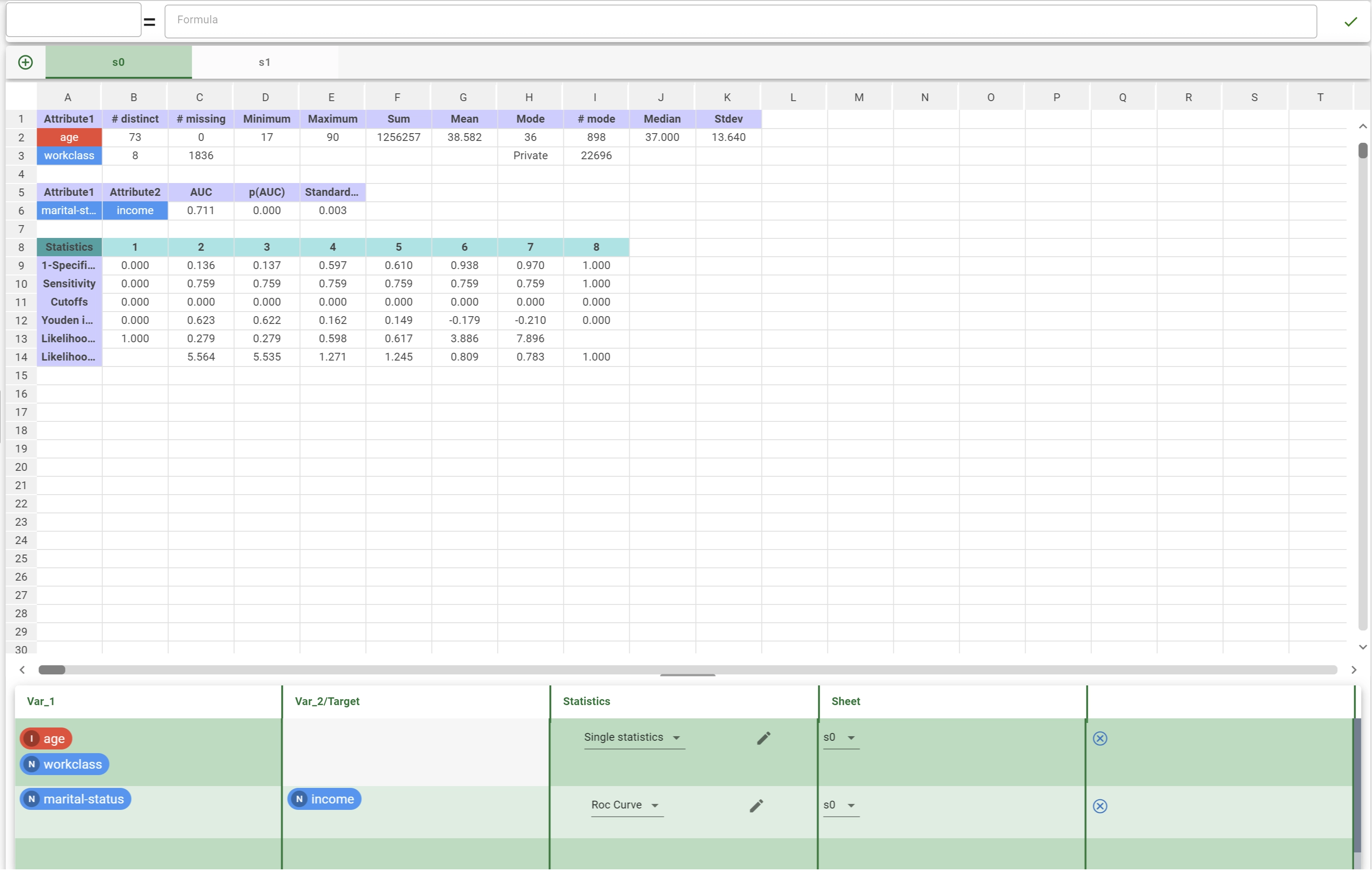
The Statistic panel
In the Statistic panel you can evaluate univariate or bivariate statistics on your data and automatically populate your sheets with the results.
Warning
Results can only be inserted on Locked sheets. If no Locked sheets are present the Statistic panel panel will be disabled.
Inputs for your statistic evaluation are provided by dragging and dropping attributes and results from the Attribute list into four different areas of the Statistic panel:
Var_1 area: controlling the main input columns for the univariate evaluation and for the statistic tests, as well as the first input columns for the bivariate evaluation and for correlation study.
Var_2/Target area: controlling the target attributes for the statistic tests, as well as the second input columns for the bivariate evaluation and for correlation study.
Statistics area: controlling the type of statistics to evaluate as well as the precise list of single statistics to include in the result representation.
Sheet area: controlling in which sheet results are displayed. The choice is only reduced to the Locked sheet list.
When attributes are dropped into the Statistic panel they are organized in rows: each row may contain an arbitrary number of attributes in each area, however, a unique table will at all times be created on the final selected sheet.
Note
Each row is associated with a unique sheet. Sheets may represent several statistics evaluated for multiple input attributes, but still only one table will be drawn. If you wish to split your evaluated stats into several Locked sheets, you are forced to split your input attributes into two separate rows of the Statistic panel.
On the right end of each filled row of the Statistic panel, a cross icon allows you to erase the whole row in a unique operation.
A complete description about the stats supported and on the internal interaction of the various four areas is available on this dedicated page.
See also
For a whole list of supported statistics and their relative types see Statistics configuration panel.