Logic Learning Machine

The Logic Learning Machine task integrates Rulex’s proprietary algorithm, called the Logic Learning Machine (or LLM, for ease in writing).

This task produces intelligible rules, like the human brain, using learned logic: this means that the algorithm needs directions provided by users to produce rules.

The output rules are produced in an if-then format.

For example:

IF weather == rain AND meeting before 9am == FALSE, THEN Best Method of Transport == Bus

This format allows users to understand and explain the logic behind predictions and makes Rulex leader in explainable AI and provides a GDPR-compliant AI tool.

The LLM task is made of three tabs:

• the Options tab

• the Monitor tab

• the Results tab

---

The Options tab

The Options tab contains all the options you can customize to obtain the desired output. It is divided itself into two tabs, the Basic and the Advanced tabs.

The Available attributes list, containing the dataset’s attributes available for the analysis, is always displayed on both tabs.

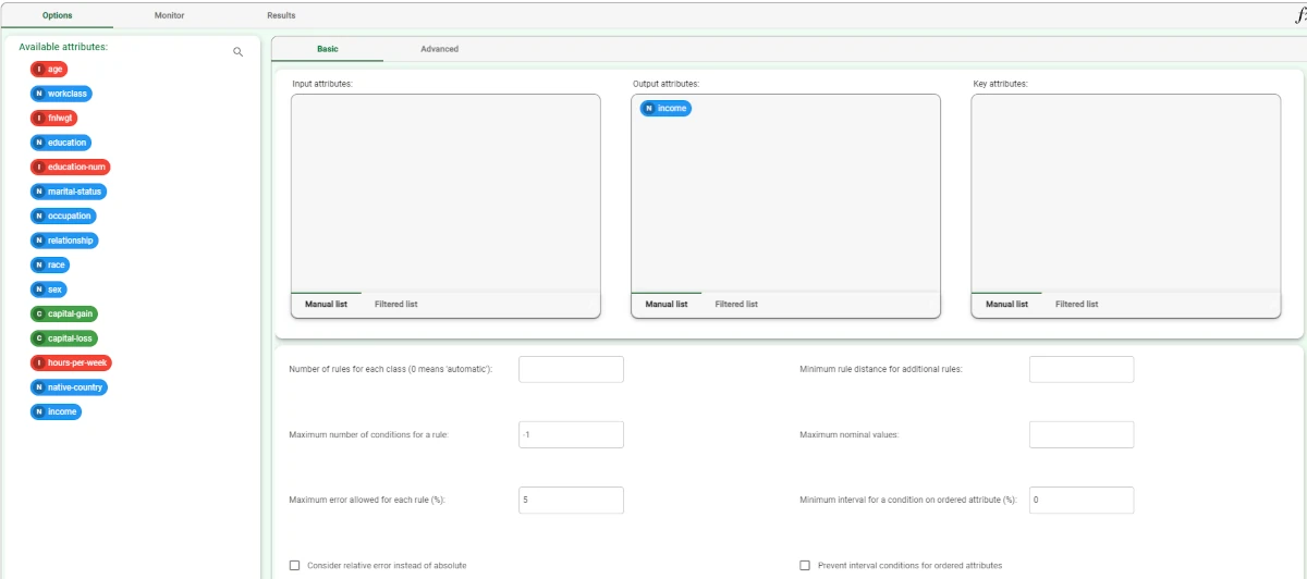
Basic

In the Basic tab, you can distinguish between three panels: the Available attributes, containing the dataset’s attributes, which can be dragged onto the second panel, the attribute drop area, to start the analysis. One last panel with general options for analysis is provided.

Drag the required attributes for analysis on the attribute drop area. The following areas are provided:

• Input attributes: the input attributes you want to use to form the rules leading to the correct classification of data. Instead of manually dragging and dropping attributes, they can be defined via a filtered list.

• Output attributes: the attributes you want to use to form the final classes into which the dataset will be divided. Instead of manually dragging and dropping attributes, they can be defined via a filtered list.

• Key attributes: the attributes that must always be taken into consideration in rules, and every rule must always contain a condition for each of the key attributes. Instead of manually dragging and dropping attributes, they can be defined via a filtered list.

The basic options panel is located under the attribute drop area and contains the following options:

• Number of rules for each class (0 means ‘automatic’): the number of rules for each class. If set to 0 the minimum number of rules required to cover all patterns in the training set is generated.

• Minimum rule distance for additional rules: the minimum difference between additional rules, taken into consideration if the Prevent interval conditions for ordered attributes option has been selected.

• Maximum number of conditions for a rule: the maximum number of conditions in a rule.

• Maximum nominal values: he maximum number of nominal values that can be contained in a condition. This is useful for simplifying conditions and making them more manageable, for example when an attribute has a very high number of possible nominal values. It is worth noting that overly complicated conditions also run the risk of over-fitting, where rules are too specific for the test data, and not generic enough to be accurate on new data.

• Maximum error allowed for each rule (%): the maximum error (in %) that a rule can score. The absolute or relative error is considered according to the whether the Consider relative error instead of absolute option is checked or not.

• Minimum interval for a condition on ordered attribute (%): the minimum interval for a condition on an ordered attribute as a percentage of the total range.

• Consider relative error instead of absolute: specify whether the relative or absolute error must be considered.
  The Maximum error allowed for each rule is set by considering proportions of samples belonging to different classes. Imagine a scenario where for given rule pertaining to the specific output value yo:

  • TP is the number of true positives (samples with the output value yo that verify the conditions of the rule).

  • TN is the number of true negatives (samples with output values different from yo that do not verify the conditions of the rule).

  • FP is the number of false positives (samples with output values different from yo that do verify the conditions of the rule).

  • FN is the number of false negatives (samples with the output values yo that do not verify the conditions of the rule).

  In this scenario the absolute error of that rule is FP/(TN+FP), whereas the relative error is obtained as follows:

  FP/Min(TP+FN, TN+FP) (samples with the output value yo that do verify the conditions of the rule).

• Prevent interval conditions for ordered attributes: if selected, interval conditions, such as 1<x≤5, are avoided, and only conditions with > (greater than) ≤ (lower or equal than) are generated.

Advanced

In the Advanced tab you can set advanced operations, which will be crucial in the overall analysis’ customization. The Available attributes list is displayed on the left, so that it is easier to work on the tab. The following options are available:

• Build rules for <all but/only> the <first/last> output value: if selected, rules only for the specified classes in this option will be created, in combination with the options only/all and first/last.

• Prevent rules in output from being included in the LLM model: if selected, rules fed into the LLM task should not be included in the final ruleset.

• Allow to use complements in conditions on nominal: if selected, conditions on nominal attributes can be expressed as complements.

• Ignore outliers while building rules: if selected, the set of remaining patterns, not covered by generated rules, are ignored if its size is less than the threshold defined in the Maximum error allowed for each rule (%) option.

• Differentiate multiple rules by attributes: if selected, when multiple rules are generated, rules which contain the same attributes in their conditions are penalized.

• Change roles for input and output attributes: if selected, input and output roles can be defined in the LLM task, overwriting the roles defined in any previous Data Manager task in the flow.

• Minimize number of conditions: if selected, rules with fewer conditions, but the same covering, are privileged.

• Ignore attributes not present in rules: if selected, attributes that have not been included in rules will be flagged Ignore at the end of the training process, to reflect their redundancy in the classification problem at hand.

• Hold all the generated rules: if selected, even redundant generated rules, which are verified only by training samples that already covered by other more powerful rules, are kept.

• Aggregate data before processing: if selected, identical patterns are aggregated and considered as a single pattern during the training phase.

• Missing values verify any rule condition: if selected, missing values will be assumed to satisfy any condition. If there is a high number of missing values, this choice can have an important impact on the outcome.

• Perform a coarse-grained training (faster): if selected, the LLM training algorithm considers the conditions with the subset of values that maximizes covering for each input attribute. Otherwise, only one value at a time is added to each condition, thus performing a more extensive search. The coarse-grained training option has the advantage of being faster than performing an extensive search.

• Allow rules with no conditions: if selected, rules with no conditions can also be generated. This may be useful, for example, if there are no examples for a specific class, as at least one rule is consequently created.

• Append results: if selected, the results of this computation are appended to the dataset, otherwise they replace the results of previous computations.

• Maximum number of trials in bottom-up mode: the number of times a bottom-up procedure can be repeated, after which a top-down procedure will be adopted.
  The bottom-up procedure starts by analyzing all possible cases, defining conditions and reducing the extension of the rules. If, at the end of this procedure, the error is higher than the value entered for the Maximum error allowed for each rule (%) option, the procedure starts again, inserting an increased penalty on the error. If the maximum number of trials is reached without obtaining a satisfactory rule, the procedure is switched to a top-down approach.

• Initialize random generator with seed: if selected, a seed, which defines the starting point in the sequence, is used during random generation operations. Consequently, using the same seed each time will make each execution reproducible. Otherwise, each execution of the same task (with same options) may produce dissimilar results due to different random numbers being generated in some phases of the process.

• Overlap between rules (%): set the maximum percentage of patterns, which can be shared by two rules.

• Key usage mode: when one or more attributes are selected as keys, the Complete value considers all the possible combinations of key values evaluating resulting conditions on the whole training set, whereas the value Partial makes this evaluation only on the portion of dataset having those key values. The value Minimal only ensures that all the generated rules include at least one condition on key attributes.

---

The Monitor tab

The Monitor tab contains statistics on the generated rules as a set of histograms. These plots can be viewed during and after the computation.

This tab is divided itself into three tabs:

• the Conditions tab

• the Covering tab

• the Error tab

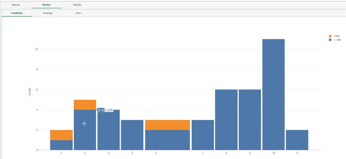
The Conditions tab

The Conditions tab contains a bar plot displaying the following information:

• On the X axis, you will find the number of conditions generated.

• On the Y axis, you will find the counts of the rules containing the specified number of conditions.

• the Color target, which can be found at the right of the plot, containing the output’s values. If you double-click on the output’s value, the plot displays the required information accordingly.

If you hover over the bars, you will find basic information on them, which generally consists of the Counts, the Range, the Color value, the Percentage on total, the Percentage on target, and the Percentage on bar.

The Covering tab

The Covering tab contains a bar plot displaying the following information:

• On the X axis, you will find the covering percentage.

• On the Y axis, you will find the counts of the rules with the corresponding percentage of covering.

• the Color target, which can be found at the right of the plot, containing the output’s values. If you click on the output’s value, the plot displays the required information accordingly.

If you hover over the bars, you will find basic information on them, which generally consists of the Counts, the Range, the Color value, the Percentage on total, the Percentage on target, and the Percentage on bar.

The Error tab

The Error tab contains a bar plot displaying the following information:

• On the X axis, you will find the error percentage.

• On the Y axis, you will find the counts of the rules with the corresponding percentage of error.

• the Color target, which can be found at the right of the plot, containing the output’s values. If you click on the output’s value, the plot displays the required information accordingly.

If you hover over the bars, you will find basic information on them, which generally consists of the Counts, the Range, the Color value, the Percentage on total, the Percentage on target, and the Percentage on bar.

---

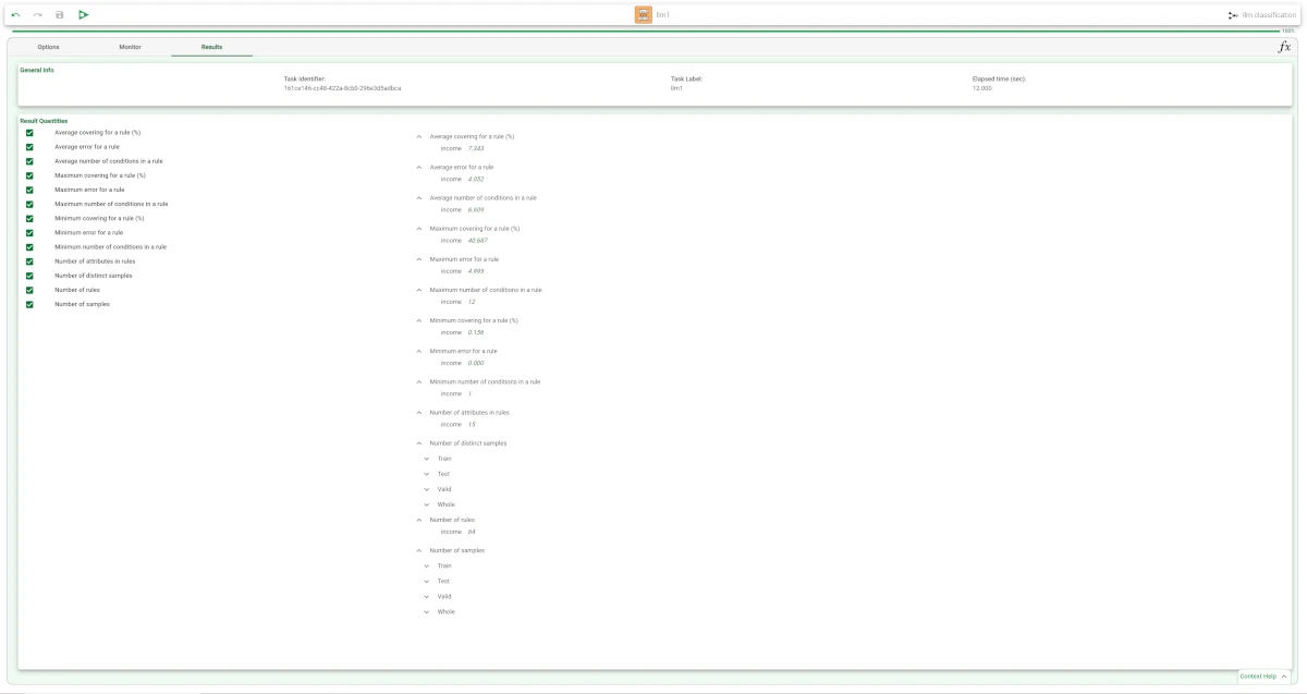
The Results tab

The Results tab provides information on the computation. It is divided into two sections:

• In the General info section you will find:

  • The Task Label, which is the task’s name on the interface.

  • The Elapsed time, which indicates how long it took to complete the computation

• In the Result Quantities panel, you will find:

  • Average covering for a rule (%)

  • Average error for a rule

  • Average number of conditions in a rule

  • Maximum error for a rule

  • Maximum number of conditions in a rule

  • Minimum covering for a rule (%)

  • Minimum error for a rule

  • Minimum number of conditions in a rule

  • Number of attributes in rules

  • Number of distinct samples

  • Number of rules

  • Number of samples

    You can check or uncheck the quantities above to visualize them in the results list. You can visualize their specific values by clicking on the arrow next to them.

---

Example

• After having imported the dataset with the Import from Text File task and splitting the dataset into test (30%) and training (70%) sets with the Split Data task, add a Classification LLM to the flow and define Income as the output attribute.

• Save and compute the task.

• Clicking on the Monitor tab displays a plot with:

  • the counts of the conditions (Conditions tab);

  • the counts of the covering (Covering tab);

  • the counts of the errors (Error tab)

• Clicking on the Results tab displays a list with:

  • the execution time (only for the LLM task),

  • some input data properties, such as the number of samples and attributes

  • some results of the computation, such as number of rules and rule statistics.

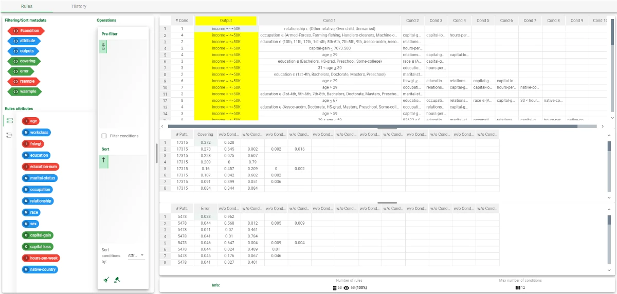
• To view the rules, add a Rule Manager task and link it to the LLM. Then, compute the Rule Manager.

• Open the task and see the results:

  • For example, rule 1 states that if relationship is Other-relative, Own-child, Unmarried then income is ≤50K.

  • The maximum covering value of rule 1 is 0.372 %, whereas the error is around 0.038 %.

  • In contrast, rule 38 asserts that if workclass is Federal-gov or Self-emp-inc then income is >50K.

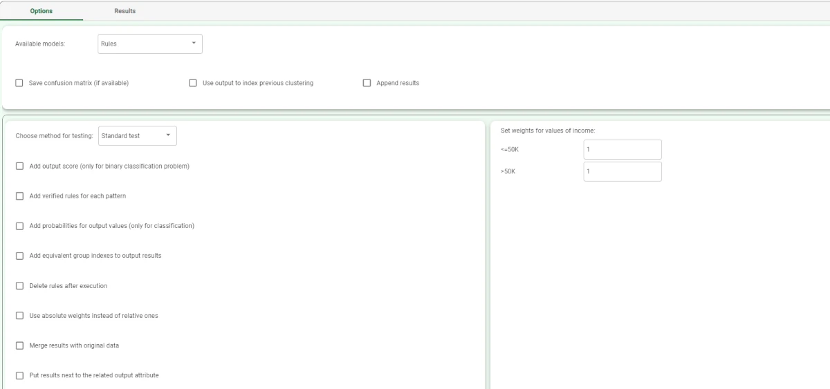
• The forecast ability of the set of generated rules can be viewed by adding an Apply Model task to the LLM task, and computing with default options.

• If required, here we could apply weights to the execution, for example if we were more interested in identifying one of the two classes.

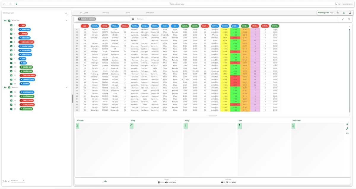
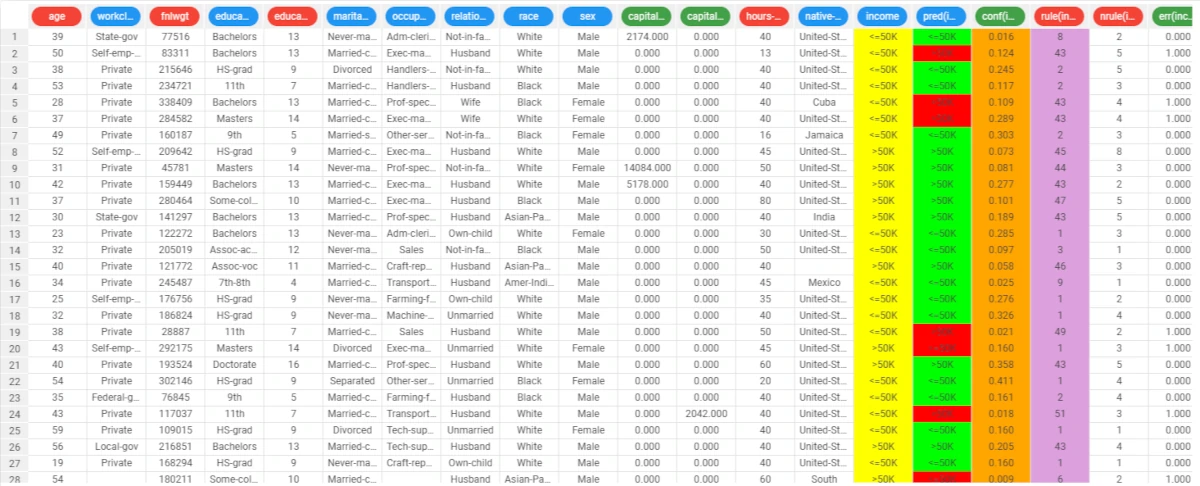
• Now right-click the Apply Model task, and select Take a look to view the results.

• The application of the rules generated by LLM has added four columns containing:

  • the forecast for each pattern: pred(income)

  • the confidence relative to this forecast: conf(income)

  • the number of rules used to make the prediction rule(income)

  • the number of the most important rule that determined the prediction: nrule(income)

  • the forecast error, i.e. 1.000 in case of misclassification and 0.000 in case of correct forecast : err(income).

• The content of the parentheses is the name of the variable the prediction refers to.

Note

Misclassified and correctly classified Correctly classified patterns are highlighted in green in the pred column and identified by the number 0.000 in the err column.

Incorrectly classified patterns are highlighted in red in the pred column and identified by the number 1.000 in the err column.

From the summary panel on the left we can see that 81.174% of patterns have been correctly classified in the training set. Note that LLM does not reach the 100% because a certain number of errors were allowed in the training phase.

• Selecting Test Set from the Displayed data drop down list shows how the rules behave on new data.

• In the test set, the percentage of accuracy is about 80.7%.

• Post-processing model optimization can improve test set accuracy (potentially) at the expense of a slightly higher error level on the training set.