Decision Tree
The Decision Tree task can solve classification problems by building a tree structure of intelligible rules.
There is a root node, which is dividing into branches, each one of them with their leaves and terminal nodes.
The task is divided into three tabs:
the Options tab
the Monitor tab
the Results tab
The Options tab
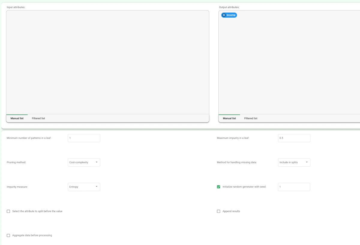
The Options tab contains all the options you can customize to perform the analysis.
It is divided into three main sections:
The Available attributes section, where you will find the dataset’s attributes, which can be dragged onto the attribute drop area. To know more about this list, go to the corresponding page.
The attribute drop area, where you can drag the attributes. Instead of manually dragging and dropping attributes onto the Input attributes and Output attributes, they can be defined via a filtered list.
- The last panel contains the customization options available:
Minimum number of patterns in a leaf: the minimum number of patterns that a leaf can contain. If a node contains less than this threshold, tree growth is stopped and the node is considered a leaf.
Maximum impurity in a leaf: specify the threshold on the maximum impurity in a node. The impurity is calculated with the method selected in the Impurity measure option.
By default this value is zero, so trees grow until a pure node is obtained (if possible with training set data) and no ambiguities remain.Pruning method: the method used to prune redundant leaves after tree creation. The following choices are currently available:
No pruning: leaves are not pruned, so the tree is left unchanged.
Cost-complexity (default value): according to this approach, implemented in CART the tree is pruned through a cost-complexity measure that creates a sequence of subtrees and finds the best one through the application on a validation set. Each subtree is created from the previous one by minimizing a cost-complexity measure that takes into account both the misclassification level in the training set and the number of leaves.
Reduced error: this simple method, introduced by Quinlan, employs the validation set to decide whether a subtree should be replaced by a single leaf. If the error in the validation set after transforming an internal node into a leaf decreases, the relative subtree is removed.
Pessimistic: the tree is based according to the pessimistic pruning approach introduced by Quinlan. Using this method it is not necessary to create a validation set since the training set is employed both for tree creation and for tree pruning. Pessimistic pruning makes use of a correction for the error rate (pessimistic error) at each node to decide whether it is to be pruned or not.
Method for handling missing data: select the method to be used to handle missing data:
Replace with average: missing values are replaced with the value fixed by the user for the corresponding attribute (for example, by means of a Data Manager). If this value is not set, the average computed on the training set is employed.
Include in splits: patterns with missing values in the test attribute at a given node are sent to both the sub-nodes deriving from the split.
Remove from splits: patterns with missing value in the test attribute are removed from the subsequent nodes.
Impurity measure: the method used to measure the impurity of a leaf. Considering a classification problem with c classes and a given node η, the following choices are currently available: Entropy, Gini, Error.
Initialize random generator with seed: if selected, a seed, which defines the starting point in the sequence, is used during random generation operations. Consequently, using the same seed each time will make each execution reproducible. Otherwise, each execution of the same task (with same options) may produce dissimilar results due to different random numbers being generated in some phases of the process.
Select the attribute to split before the value: if selected, the QUEST method is used to select the best split. According to this approach, the best attribute to split is selected via a correlation measure, such as F-test or Chi-Square. After choosing the best attribute, the best value for splitting is selected.
Append results: if selected, the results of this computation are appended to the dataset, otherwise they replace the results of previous computations.
Aggregate data before processing: if selected, identical patterns are aggregated and considered as a single pattern during the training phase.
Maximum depth: set the maximum depth of the tree conditions.
The Monitor tab
The Monitor tab contains statistics on the generated rules as a set of histograms. These plots can be viewed during and after the computation.
This tab is divided itself into three tabs:
the Conditions tab
the Covering tab
the Error tab
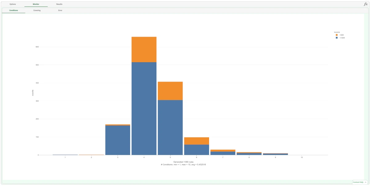
The Conditions tab
The Conditions tab contains a bar plot displaying the following information:
On the X axis, you will find the number of conditions generated.
On the Y axis, you will find the counts of the rules containing the specified number of conditions.
the Color target, which can be found at the right of the plot, containing the output’s values. If you click on the output’s value, the plot displays the required information accordingly.
If you hover over the bars, you will find basic information on them, which generally consists of the Counts, the Range, the Color value, the Percentage on total, the Percentage on target, and the Percentage on bar.
The Covering tab
The Covering tab contains a bar plot displaying the following information:
On the X axis, you will find the covering percentage.
On the Y axis, you will find the counts of the rules with the corresponding percentage of covering.
the Color target, which can be found at the right of the plot, containing the output’s values. If you click on the output’s value, the plot displays the required information accordingly.
If you hover over the bars, you will find basic information on them, which generally consists of the Counts, the Range, the Color value, the Percentage on total, the Percentage on target, and the Percentage on bar.
The Error tab
The Error tab contains a bar plot displaying the following information:
On the X axis, you will find the error percentage.
On the Y axis, you will find the counts of the rules with the corresponding percentage of error.
the Color target, which can be found at the right of the plot, containing the output’s values. If you click on the output’s value, the plot displays the required information accordingly.
If you hover over the bars, you will find basic information on them, which generally consists of the Counts, the Range, the Color value, the Percentage on total, the Percentage on target, and the Percentage on bar.
The Results tab
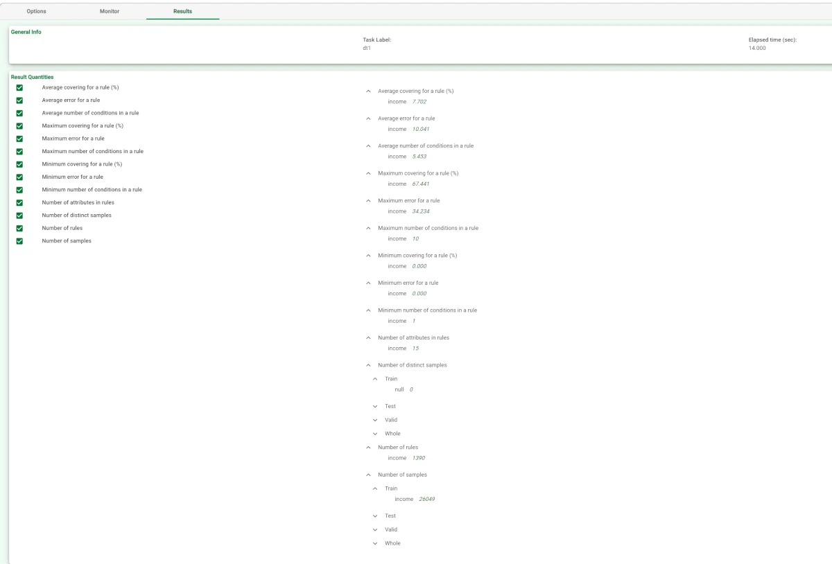
The results tab provides information on the computation. It is divided into two sections:
- In the General info section you will find:
The Task Label, which is the task’s name on the interface.
The Elapsed time, which indicates how long it took to complete the computation
- In the Result Quantities panel, you will find:
Average covering for a rule (%)
Average error for a rule
Average number of conditions in a rule
Maximum error for a rule
Maximum number of conditions in a rule
Minimum covering for a rule (%)
Minimum error for a rule
Minimum number of conditions in a rule
Number of attributes in rules
Number of distinct samples
Number of rules
Number of samples
You can check or uncheck the quantities above to visualize them in the results list. You can visualize their specific values by clicking on the arrow next to them.
Example
After importing the adult dataset with the Import from Text File task and splitting the dataset into test and training sets (20% test, 20% validation and 60% training) with the Split Data task, add a Decision Tree task to the process and double-click the task.
- Select:
Cost-complexity as pruning method
0.5 as Maximum impurity in a leaf
Income as the output attribute
Compute the task to start the analysis.
The properties of the generated rules can be viewed in the Monitor tab of the Decision Tree task:
There are, for example, 656 rules with 4 conditions, 515 relative to class “<50K, and 141 relative to class “>50K”.
The total number of rules, and the minimum, maximum and average of the number of conditions is reported, too.
Analogous histograms can be viewed for covering and error, by clicking on the corresponding tabs.
- Clicking on the Results tab displays a spreadsheet with:
the execution time (only for the DT task),
some input data properties, such as the number of patterns and attributes
some results of the computation, such as number of rules and rule statistics.
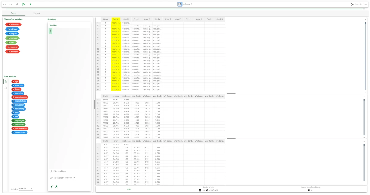
The rule spreadsheet then can be viewed by adding a Rule Manager task.
Each row displays all the conditions that belong to the specific rule.
The total number of generated rules is 1390, with a number of conditions ranging from 1 to 10.
The maximum covering value is 67.4%, whereas the maximum error is about 15%.
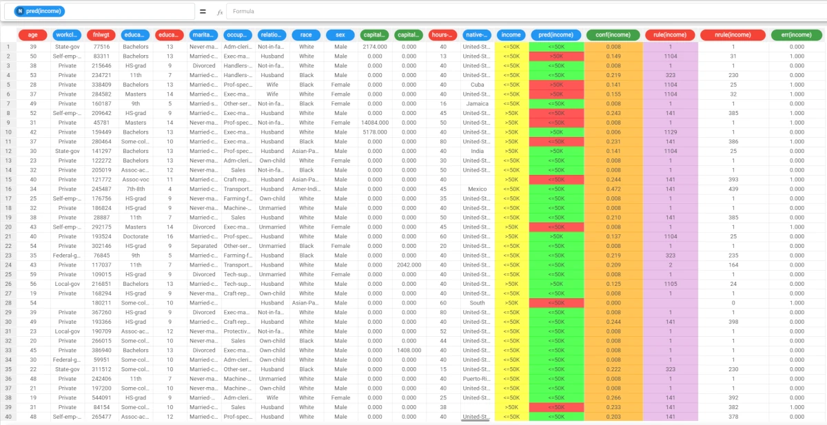
We can check out the application of this set of rules to the training and test patterns by right-clicking the Apply Model task and selecting Take a look.
- The application of the rules generated by the Decision Tree task has added new columns containing:
the forecast for each pattern: pred(income)
the confidence relative to this forecast: conf(income)
the number of rules used by each pattern rule(income)
the most important rule that determined the prediction: nrule(income)
the classification error, i.e. 1 if misclassified and 0 if correctly classified: err(income).