Neural Networks

The classification Neural Networks task builds a feed-forward neural network (NN) for classification. NN is a model that includes a certain number of elementary perceptrons organized in layers.

The layers can be distinguished into three groups:

• Input layer, from which the Neural Network receives the data. The number of neurons in this group corresponds to the number of inputs.

• Output layer, containing the analysis’ output. The number of neurons in this group corresponds to the possible classes.

• Hidden layers, located between the input and the output layers.

Each perceptron returns sigmoid function (activation function) that depends on a weighted sum of its input. To retrieve the optimal weight vector for each perceptron a back-propagation algorithm is employed.

The output of the task is a model, consisting in a weight matrix, that can be employed by an Apply Model task to perform the NN forecast on a set of examples.

The task is divided into four tabs:

• the Options tab

• the Monitor tab

• the Weights tab

• the Results tab

---

The Options tab

The Options tab contains all the options you can customize to perform the analysis.

It is divided itself into two tabs, the Basic and the Advanced tabs.

The Available attributes list, containing the dataset’s attributes available for the analysis, is always displayed on both tabs.

Basic

In the Basic tab, you can distinguish between three panels: the Available attributes, containing the dataset’s attributes, which can be dragged onto the second panel, the attribute drop area, to start the analysis. More information on the available attributes and the One last panel with general options for analysis is provided.

Drag the required attributes for analysis on the attribute drop area. The following areas are provided:

• Input attributes: the input attributes you want to use to form the rules leading to the correct classification of data. Instead of manually dragging and dropping attributes, they can be defined via a filtered list.

• Output attributes: the attributes you want to use to form the final classes into which the dataset will be divided. Instead of manually dragging and dropping attributes, they can be defined via a filtered list.

• The last panel contains the customization options available:

  • Number of hidden layers: the number of hidden layers in the network.

  • Neurons for each hidden layer: the number of neurons in each hidden layer. This option is enabled only if the value specified for the Number of hidden layers option is greater than zero.

  • Learning rate: indicate the coefficient of the gradient descent. For high values it is likely that the algorithm converges more quickly, but it may lack in precision. Alternatively, with low learning rates, the algorithm will converge more slowly, but with more accuracy.

  • Momentum term: specify the momentum of the back-propagation algorithm. Momentum adds a fraction (between 0 and 1) of the previous weight update to prevent the system from converging to a local minimum.

  • Normalization for input attributes: the type of normalization to use when treating ordered (discrete or continuous) variables. Possible methods are:

    • None: no normalization is performed.

    • Attribute: the normalization is performed following the normalization set for each attribute in the previous Data Manager.

    • Normal: data are normalized according to the Gaussian distribution, where μ is the average of x and σ is its standard deviation.

    • Minmax [0,1]: data are normalized to be comprised in the range [0,1].

    • Minmax [-1,1] (default): data are normalized to be included in the range [-1, 1].

    Every attribute can have its own value for this option, which can be set in the Data Manager task.
    These choices are preserved if Attribute is selected in the Normalization of input variables option; otherwise any selections made here overwrite previous selections made.

  • Normalization for output attributes: select the method for normalizing output variables. Possible methods are:

    • None: no normalization is performed.

    • Attribute:

    • Normal: data are normalized according to the Gaussian distribution, where μ is the average of x and σ is its standard deviation.

    • Minmax [0,1]: data are normalized to be comprised in the range [0,1].

    • Minmax [-1,1] (default): data are normalized to be included in the range [-1, 1].

    Every attribute can have its own value for this option, which can be set in the Data Manager task.
    These choices are preserved if Attribute is selected in the Normalization of output variables option; otherwise any selections made here overwrite previous selections made.

Advanced

In the Advanced tab, you will find the following customization options, along with the Available attributes list:

• Maximum number of iterations: the maximum number of iterations allowed for the gradient descent algorithm for each trial.

• Number of trials: select the number of trials, i.e. the repeated execution of back-propagation algorithm, with different starting conditions.

• Maximum number of iterations for any trial: the maximum number of iterations allowed for the gradient descent algorithm for each trial.

• Initialize random generator with seed: if selected, a seed, which defines the starting point in the sequence, is used during random generation operations. Consequently, using the same seed each time will make each execution reproducible. Otherwise, each execution of the same task (with same options) may produce dissimilar results due to different random numbers being generated in some phases of the process.

• Use symmetric activation function: if selected, use an activation function in the range (-1,1) instead of (0,1).

• Append results: if selected, the results of this computation are appended to the dataset, otherwise they replace the results of previous computations.

• Aggregate data before processing: if selected, identical patterns are aggregated and considered as a single pattern during the training phase.

---

The Monitor tab

In the Monitor tab it is possible to view the temporal evolution of some quantities related to the network optimization.

It is divided into three tabs: the Error, the Gradient and the Misclassified tabs: their behavior is reported as a function of the number of iterations.

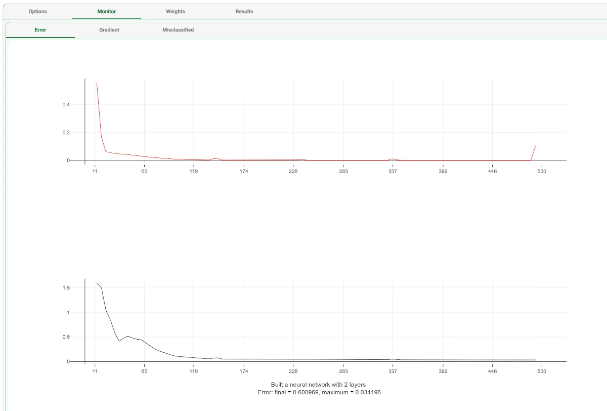
Each tab contains two curve plots: the first plot displays the error’s mean, calculated on the training set, while the second plot displays how the maximum error value varies during the algorithm iterations.

These plots can be viewed during and after computation operations.

In all tabs, the X axis displays the number of iterations, while the Y axis displays the Error/Gradient/Misclassified value at every iteration.

---

The Weights tab

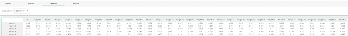
In the Weights tab it is possible to view the weight matrix for each hidden layer.

The layer to be displayed can be selected from the Choose Layer drop down list.

Each row in the spreadsheet represents a neuron, while the first column contains the Bias for each neuron, and the following ones contain the Weights.

Note

The bias is a constant which gets added to the product of features and weights. It helps to shift the model towards the positive or negative side.

The weights are values telling the importance of each input.

---

The Results tab

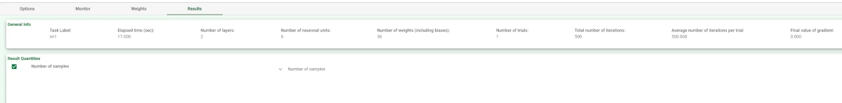
The results tab provides information on the computation. It is divided into two sections:

• In the General info section you will find:

  • The Task Label, which is the task’s name on the interface.

  • The Elapsed time, which indicates how long it took to complete the computation.

  • The Number of layers, which indicates the total (hidden and output) layers.

  • The Number of neuronal units.

  • The Number of weights (including biases).

  • The Number of trials.

  • The Total number of iterations.

  • The Average number of iterations per trial.

  • The Final value of gradient.

• In the Result Quantities section, you will find:

  • The Number of samples obtained, divided by the following sets:

    • Train

    • Test

    • Valid

    • Whole

---

Example

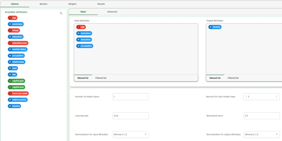
• After having imported the dataset with the Import from Text File task and splitting the dataset into test and training sets (30% test and 70% training) with the Split Data task, add a Neural Networks to the flow and configure the NN task as follows:

  • Number of hidden layers: 1

  • Neurons for each hidden layer: 5

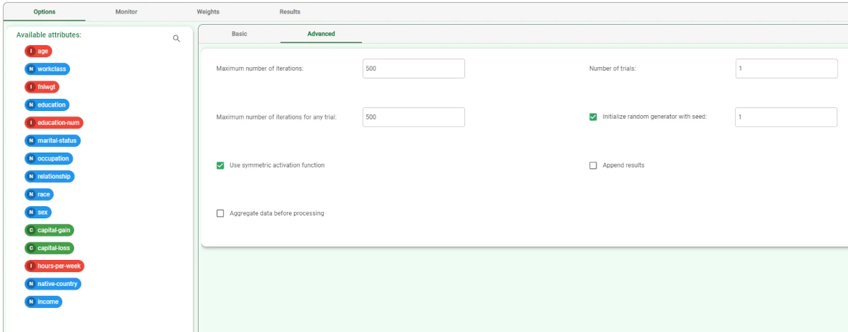
  • Maximum number of iterations: 500

  • Maximum number of iterations for any trial: 500

  • Income attributes: age, workclass, education, occupation.

  • Output attributes: income.

• Leave the other options with their default values and compute the task.

• The execution of the task can be monitored in the Monitor tab of the NN task. In these plots the behavior of the error as a function of the iteration is showed. Analogous plots can be visualized for gradient and misclassified by clicking on the corresponding tabs.

• Clicking on the Weights tab at the end of the execution, displays the weights obtained through the optimization procedure. The layer to be visualized can be selected in the Select a layer drop-down list. Each row corresponds to a neuron of that layer and contains the weights relative to each input attribute. The first column contains the bias, i.e. the constant term in the linear combination of inputs.

• The Results tab contains a summary of the computation.

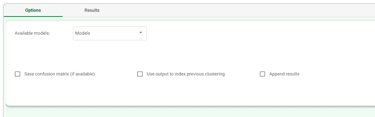
• The forecast ability of the set of generated rules can be viewed by adding an Apply Model task to the Neural Networks task, and computing with default options.

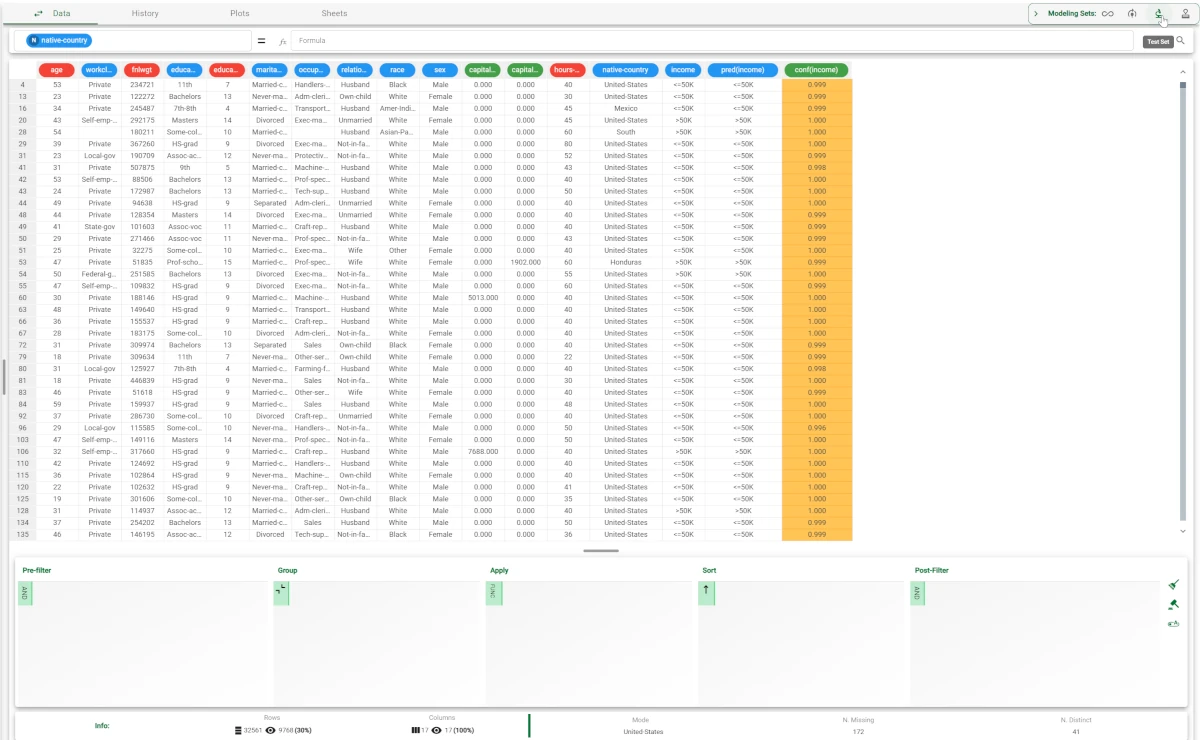
• The forecast produced by the Apply Model task can be analyzed by right-clicking the task and selecting Take a look.
  In the data table the following columns relative to the results of the elaboration have been added:

  • the NN output forecast: pred(income)

  • the confidence of this forecast: conf(income)

• Selecting Test Set from the Displayed data drop down list shows how the rules behave on new data.

• Selecting Test Set from the Displayed data drop down list shows how the rules behave on new data.