Build and Solve

Warning

This task is available on specific request only. Contact us for specific pricing.

The Build/Solve task constructs and solves an optimization problem. This task requires two input files:

• a dataset showing the problem’s features, which doesn’t need to have a specific structure, it only needs to contain a row for each possible solution.

• a configuration file, defining the constraints of the problem. A full description of the configuration file, along with its features and syntax is provided in the corresponding section.

After having prepared the configuration file following the provided guidelines, the task itself has a simple configuration layout, made of the Options tab only.

---

The Options tab

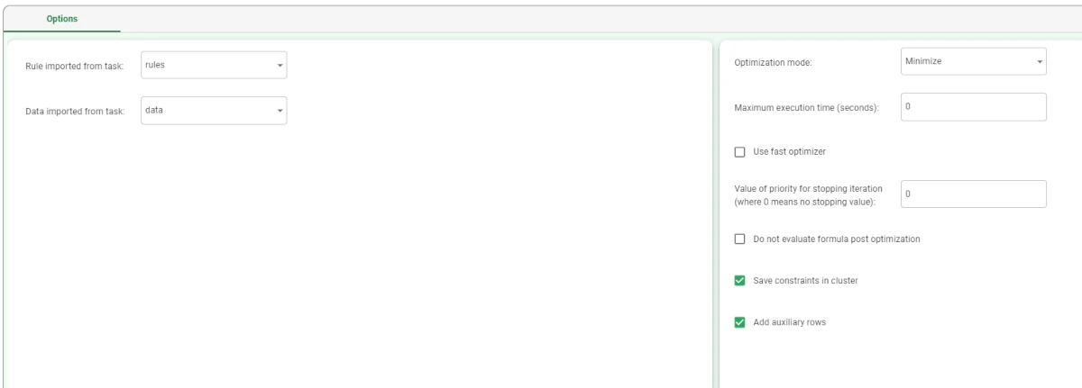
The Build/Solve task requires two input tasks: one containing the problem’s features, and another containing the optimization constraints. When opening the Build/Solve task, the Options tab is the only tab available.

It is divided into two areas:

• in the left one, users must define the tasks containing the problem’s description and the configuration file. This is possible through the following options:

  • Rule imported from task: specify the task containing the file with the constraints’ definition.

  • Data imported from task: specify the task containing the file with the details which make up the problem.

• in the area located on the right, users can customize the optimization features through the following options:

  • Optimization mode: specify the solution’s outcome. The possible values are:

    • Minimize (default)

    • Maximize

  • Maximum execution time (seconds): specify the execution’s time limit in seconds. If not specified, no limits are set.

  • Value of priority for stopping iteration (where 0 means no stopping value): the priority value where the loop on the priority will be stopped. If not specified, the loop doesn’t stop.

  • Do not evaluate formula post optimization: if selected, the formulas with the after Application value in the configuration file will not be evaluated when stopping the priority evaluation.

  • Save constraints in cluster: if selected, the sparse input matrix will be saved in a cluster structure. This structure can be visualized by importing it through an Import from Task task.

  • Add auxiliary rows: if selected, auxiliary rows will be added to the output dataset. The auxiliary rows provide information on the auxiliary variables, which have been defined in the configuration file and added during the optimization process.

  • Solver used for optimization: select the solver which will be used for the optimization operation. Possible solvers are:

    • Coin-Or: it is a collection of interoperable open source solvers from the repository of open source software maintained by the COIN-OR Foundation. More information can be found in the website.

    • Symphony: it is an open-source generic MILP solver, callable library, and extensible framework for implementing customized solvers for mixed-integer linear programs (MILPs). More information can be found in the website.

    • Naive (Rulex proprietary solver, it is faster than the others, but it provides a less accurate result)

  • Stop at first feasible solution: if selected, the optimization operation stops when a solution satisfying all the constraints is found. It might be possible that the solution found is not the best one.

  • Add feasible column in dataset: if selected, a binary column, called ‘Feasible’ is added to the dataset. The value True indicates that the solution is feasible, while the value False indicates that the solution is unfeasible.

---

The Constraints Configuration File

The configuration file must follow a strict setup: it can have any format, (the most commonly used is MS Excel) and it must have two sheets, each of them containing specific information:

• the first sheet contains the variables definition,

• the second sheet contains the constraints definition.

Warning

The sheets must follow the order listed above, otherwise the optimization operation won’t make sense.

Tip

The two sheets don’t need to have a specific name, so users can choose the one which fits better according to their needs.

Sheet 1 - Variables definition

The first sheet of the configuration file is the one defining variables. The system will check if the specified attributes satisfy the specified features. The more variables are specified and described, the more precise and reliable will be the optimization output. The sheet name can be customized by the user. The first sheet must contain the following columns:

• For (optional): definition of a group of variables. It creates n variables, where n is the number of values of the list. The syntax which must be used is @variable_name in [list_of_values]. A formula can also be inserted in the list_of_values field. If the variable is mentioned in the Formula field, it allows creating multiple formulas (according to what has been specified in this field) by simply adding the variables in the formula itself. If the variable is mentioned in the Attribute field, it creates as many attributes as the number of values in the list.

• Attribute: the name of the attribute which is being defined as a variable. Specify also the attributes which need to be added to the dataset and defined in the Formula column.

• Role: the role the corresponding attribute is going to play in the optimization process. The possible values are:

  • Key: the task verifies that the attribute is a key. The task checks that each row of the key attribute has a different value. More than one attribute can be specified.

  • Input: attributes containing important information to solve the optimization problem.

  • Solution (mandatory): variable representing the solution. This role must be specified.

  • Cost: the cost associated to each solution. It indicates the cost value of only one unit of the Solution.

  • Priority: the priority value associated to each row. The corresponding attribute’s type must be integer, with positive values only, where the value 1 indicates the highest priority, 2 a priority lower than 1, and so on.

  • Type: the type of the solution generated by the task. If this role is not specified, the type will be taken from the Solution attribute. As the Solution attribute is usually empty, its type can be customized using a Data Manager, before the Build/solve task and linked one to each other. The values in the corresponding Attribute can be:

    • 0: continuous solution

    • 1: integer solution

    • 2: binary solution

  • Minimum: the solution’s minimum value. If not specified, its value is 0.

  • Maximum: the solution’s maximum value. If not specified, its value is infinite.

• Distinct (optional): the system checks that the attributes specified in the Attribute column values is constant for each attribute value in the Distinct column. More than one attribute can be specified, so the system checks that the attribute is constant for the associated group values. If they are not constant, the system raises an error.

• Formula (optional): here, any Data Manager formula can be inserted, as well as the IF, THEN, ELSE rule. The results of these formulas will then be used to fill the attribute specified in the Attribute column. This field can be used to define new attributes that must be added to the problems’ dataset when they are not already present. These variables depend on the inputs defined in the Roles column.

• Application (optional): if a sequence of formulas must be applied, the priority can be specified in this column. The possible values are:

  • (missing value)/ start: if the value is left empty, the evaluation is performed only once, before starting the optimization.

  • before: the variable-formula is calculated at each iteration, before the optimization process.

  • after: the variable-formula is calculated after the end of the optimization process.

  • end: the variable-formula is calculated only once, after the end of the optimization process.

• Description (optional): a description of the defined variable in natural language. Users can add any description to better understand the variable’s features.

• Priority (optional): since the priority can be dynamic, this column contains integer numbers defining when functions and constraints in the corresponding row must be calculated while the specified priority is being evaluated by the Build/Solve task.

See also

As said while defining the Formula column, the if, then, else rule can be added. Its syntax is: if condition(s) then true (i.e. the value to display if the condition is satisfied) else false (i.e. the value to display if the condition is not satisfied).

If it is necessary to insert functions in the if then else constraints, it is required to use the ifelse() function. More information on the ifelse function can be found in the corresponding page.

See also

The variables which have their role set as Solution must be used alone or inside a sum or a sumIf function.

The sumIf function follows the syntax: sumIf(var_name, condition). This function performs the sum only when the specified condition is verified.

For example, sumIf($"att_1", $"att_2" > 0) means that the att_1 values will be summed only in the rows where $"att_2" > 0.

---

Sheet 2 - Constraints definition

The second sheet defines the constraints which must be taken into consideration when the task performs the analysis.

As previously said, the sheet’s name can be customized by the user, but it must contain the following columns:

• For (optional): definition of a group of constraints. It creates n constraints, where n is the number of values of the list. The syntax which must be used is @variable_name in [list_of_values]. A formula can also be inserted in the list_of_values field. If the variable is inserted in the Constraint field, it allows creating multiple constraints (according to what has been specified in this field) by simply adding the variables in the constraint itself. This way, it is possible to include the group in a unique constraint, without creating multiple ones.

• Constraint: definition of the constraint using Rulex syntax. Two types of constraints can be added, depending on their aim:

  • variable’s definition: as there are some variables which depend on the solution, and are calculated during the analysis, these constraints define the new attribute starting from the solution. These constraints must be created using the define keyword in the rule. Once created, the defined variable can be used in other constraints.

  • constraints: they are constraints which are applied to the existing variable-solutions or to solution dependent variables. These constraints must be created using the let keyword in the rule.

• Description (optional): a description of the constraint in natural language. Users can add any description to better understand the constraint’s features.

More information on keywords and on the constraints’ syntax is provided in the paragraph below.

---

Constraints syntax

The following keywords must be taken into consideration while writing a constraint, as each one of them gives specific directions to the system to calculate the best solution:

Keyword	Description	Example
when	It works as a filter, it specifies the object’s features. It is possible to use all the Data Manager conditions.	when $"Att_1" < "5"
foreach	It is used to check a group’s values. Attributes specified after the foreach keyword are used to divide the dataset values in groups, and a constraint for each group of values.	foreach $"Attr_1" foreach ($"Att_1",$"Att_2")
forevery	When it is used to check ordered attributes, it emulates the behavior of a moving window made of the number of values specified in the overlap parameter of the chosen attribute. The number specified after the forevery keyword indicates the number of values of the moving window. When it is used to check nominal attributes, it evaluates all the possible combinations, without repeating them: for example, if the combination A, B has already been evaluated, the combination B A won’t be taken into consideration.	forevery 3 $"quantity" overlap 2 (ordered values in the $"quantity" attribute) forevery 2 $"material" (when nominal values are present in the $"material" attribute)
overlap	It specifies the shift values of the ordered attributes checked with the forevery parameter. Its values must be ordered only.	forevery 3 $"quantity" overlap 2
define	It introduces an auxiliary variable definition.	define $"UseDest" = sum($"Moved") >= 1
let	It introduces a constraint. A constraint must contain a comparison operator. The variables which have their role set as Solution must be located on the left of the comparison operator, while the variables which are not Solution must be located on the right of the comparison operator. The left-hand-side element of the constraint must be linear in its variables, so it can only contain a sum or a difference between them.	let sum($"Moved") <= max($"New(Supply)"

The keywords listed below are auxiliary ones, so they are not mandatory.

Keyword	Description	Example
cost (evaluated when the keyword let or define is present)	It is the cost related to the corresponding constraint. When a define statement is present, it is the unit cost of the auxiliary variable. In the other cases, it is the cost of the constraint that is added to the overall cost when the constraint is violated. A Data Manager formula can be inserted.	cost $"DestCost"
minimum (evaluated when the keyword define is present)	It is the auxiliary variable’s minimum value. A Data Manager formula can be inserted.	minimum 0 minimum mean ($"cost")
maximum (evaluated when the keyword define is present)	It is the auxiliary variable’s maximum value. A Data Manager formula can be inserted.	maximum 8 maximum max ($"cost")
tol (evaluated when the keyword let is present)	It indicates the allowed tolerance value, according to the set parameters. It indicates the allowed error, how much the constraint can be violated.	tol 4
type (evaluated when the keyword define is present)	The auxiliary variable’s type. It can be defined with a Data Manager formula or with the following values: 0: continuous type. 1: integer type. 2: binary type.	type 2

Important

While writing the constraint, the following keyword order must be followed in the string:

1. when

2. foreach

3. forevery

4. overlap (if the attribute in the forevery parameter is ordered)

5. define or let

6. all the other keywords left

See also

Two possible rules can be:

• when $"Att_1" == "A" foreach ($"Items",$"Month") define $"Attr_1 in Month" = if sum($"Solution") >= 1 then 1 else 0 maximum 1 cost 1

• when $"$January" ==1 foreach ($"Order_numer",$"Revenue") let sum($"Solution") >= $"Minimum_Revenue_January"

---

Example

This example uses the Data and Rules datasets.

As the Build/Solve task can produce not only a simple dataset containing the solution, but also auxiliary rows or the constraint matrix, this paragraph will contain both the example with the simple solution dataset and the example with the auxiliary rows and the constraints matrix.

• Import the two required datasets to perform the analysis.

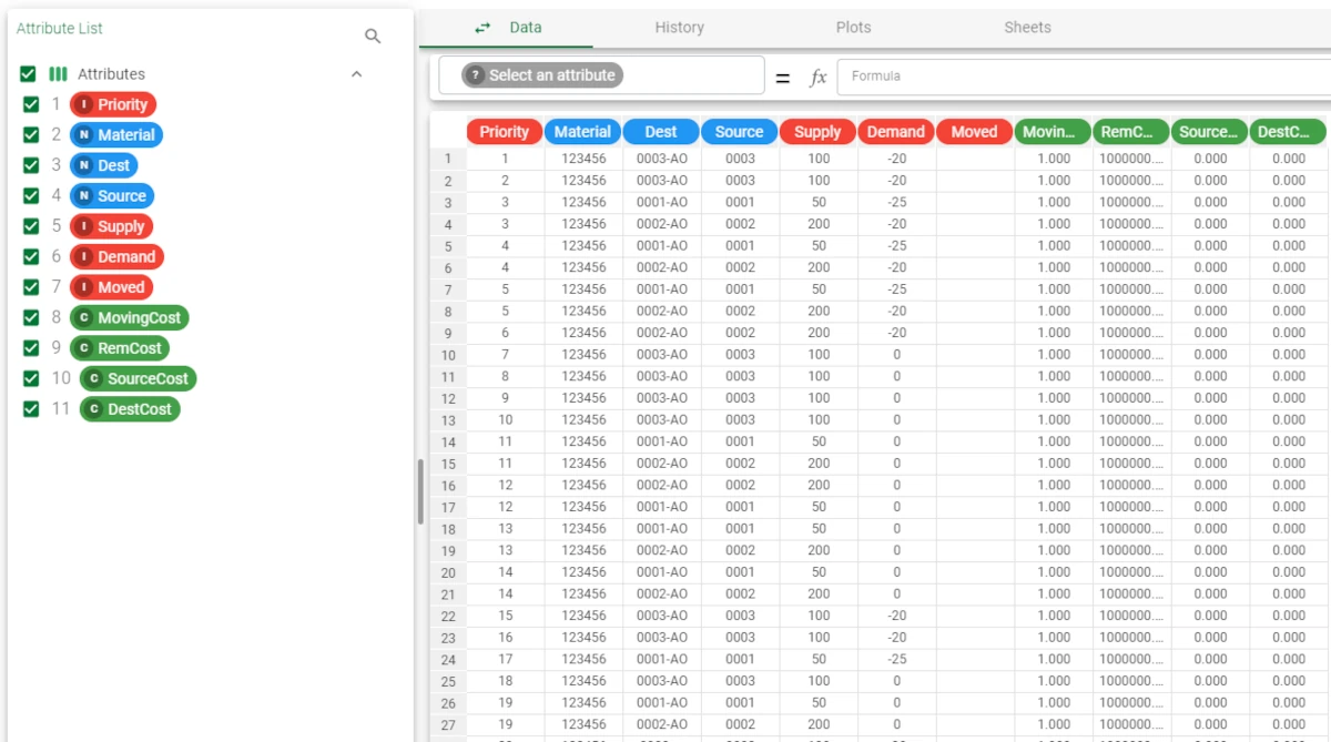
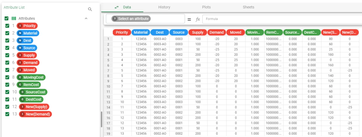
• The first dataset contains a full description of the shipping, through attributes like the Priority, the Dest, the Source and so on. You can visualize the dataset itself by opening it through a Data Manager task or by right-clicking on the import task containing it and selecting Take a Look. For ease in working in the flow, we recommend you to rename the task containing the dataset with the problem details, so that it is easily recognizable while configuring the Build/Solve task.

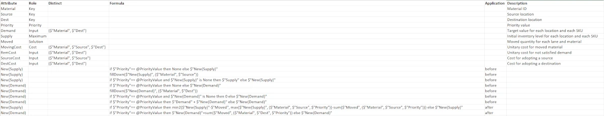
• The second dataset is the configuration file, containing the variables’ definition and the constraints. In the first sheet, the variables have been defined. For example, we can find the following definitions:

  • The Material attribute, along with the Source and Dest attributes, have been defined as Key in the Role column.

  • The Demand, MovingCost, RemCost, SourceCost and DestCost have been defined so that the system checks that the combinations written in the Distinct columns are constant.

  • The attributes located from row 13 to row 21 are calculated during the analysis: their value is defined by the function indicated in the Formula field in the configuration file, and the moment where they will be calculated is defined in the Application column. You can visualize the dataset itself by opening it through a Data Manager task or by right-clicking on the import task containing it and selecting Take a Look. For ease in working in the flow, we recommend you to rename the task containing the dataset with the problem details, so that it is easily recognizable while configuring the Build/Solve task.

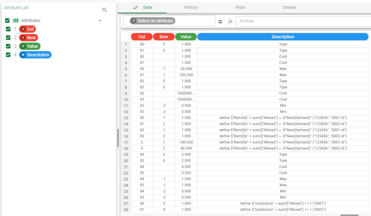
• The second sheet contains the constraints. For example:

  • The Remaining demand at destination for a given material has been defined with the following constraint: foreach ($”Material”, $”Dest”) define $”RemQty” + sum($”Moved”) = -$”New(Demand)” minimum 0 cost $”RemCost”, which means that the remaining demand must be calculated taking into account that each $”Material” and $”Dest” pair plus the sum of the $”Moved” attribute must be equal to the corresponding value of the $”New(Demand)” attribute. The minimum value for the auxiliary variable must be 0, and the cost of this solution is the $”RemCost” attribute.

  • Note that the $”New(Demand)” attribute has been evaluated before the optimization started, so it is normal not to see it in the original shipping dataset.

Simple solution dataset

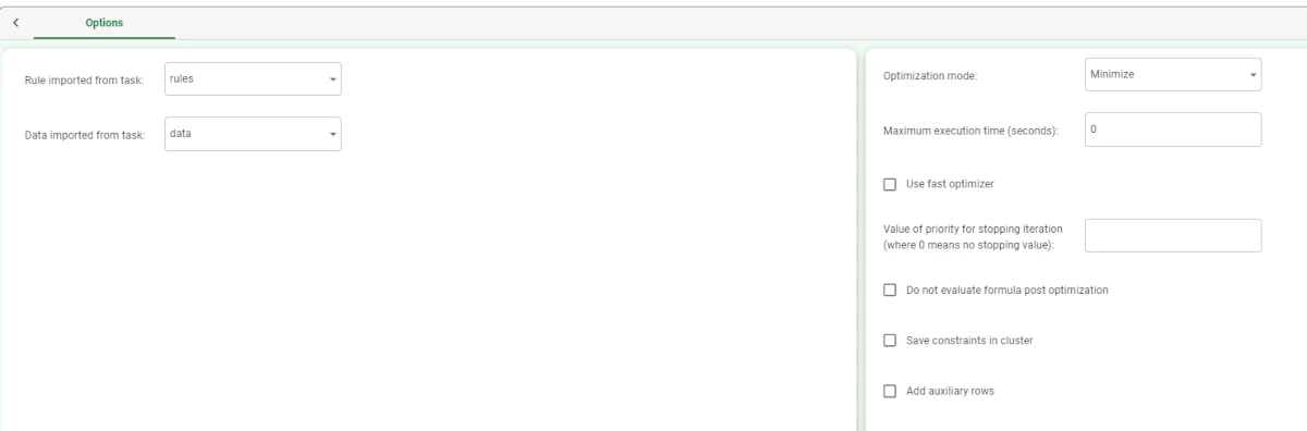
• Add a Build/Solve task, and link both datasets to it. Configure the task as follows:

  • Rule imported from task: rules (the name we gave to the task containing the configuration file)

  • Data imported from task: data (the name we gave to the task containing the shipping data which make up the problem)

  • Leave the other options as default.

  • Save and compute the task.

• Add a Data Manager task and link it to the Build/Solve task.

• Then, double-click on the Data Manager to visualize the results.

• The solution dataset has been updated with the new columns, filled with the values that are the result of the configuration file’s variables and constraints evaluation.

Auxiliary rows and constraints matrix

• After having added a Build/Solve task, configure it as follows:

  • Rule imported from task: rules (the name we gave to the task containing the configuration file)

  • Data imported from task: data (the name we gave to the task containing the shipping data which make up the problem)

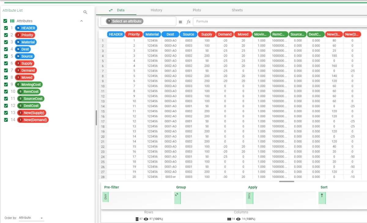
  • Check the Add auxiliary rows and the Save constraints in cluster checkboxes.

  • Save and compute the task.

• To visualize the generated solution, along with its auxiliary rows, add a Data Manager task and link it to the Build/Solve task. The dataset will have more rows, if we compare it to the solution dataset generated by leaving the configuration options untouched.

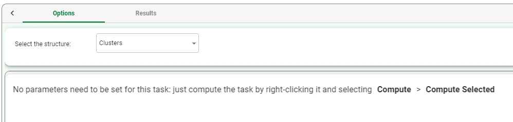
• To visualize the constraints matrix, add a Convert Structure to Dataset task and link it to the Build/Solve task.

• Open the Convert Structure to Dataset task and double check that Clusters has been selected in the Select the structure option.

• Save and compute the task.

• Add a Data Manager task and link it to the Convert Structure to Dataset task to visualize the constraints matrix.