Distribution Planner

Warning

This task is sold separately from the available licenses. Contact us for specific pricing.

The Distribution Planner task optimally manages the deployment phase in any distribution network, over any time period. It minimizes overall cost while ensuring compliance with key constraints such as delivery times, calendars, warehouse capacities, and more. Performing optimal Deployment is the aim of the Distribution Planner task.

This task calculates the best route (which will be called lane in this page) goods need to follow both minimizing transport costs and fulfilling the demand for destination nodes in the required timeframe.

Note

The Distribution Planner task ensures that the attributes defining the source and the destination are consistent. It performs two checks:

• The task verifies that the attributes defining the source and destination are equal in number and compatible in type, based on the links connecting all source-destination pairs. As a source node can also be a destination, they must be encoded in the same way.

• The task verifies that, for a given date, the quantity of material specified in a source node remains consistent across all rows in which that node appears. In such cases, the task verifies that the demand for the given date remains consistent across all rows in which it appears.

More specifically, if the same node also functions as a destination, its associated value may differ from the value it has when defined as a source.

The task produces three columns as output, which are added at the end of the output dataset:

• moved, containing the amount of goods moved.

• new(source_quantity_attribute), containing the amount of goods remaining in the source location.

• new(destination_quantity_attribute), containing the amount of goods now in the target location.

The Distribution Planner task has two tabs:

• the Options tab, where users can customize the available options to obtain the desired output.

• the Results tab, where users can visualize the computation results.

---

The Options tab

The Options tab contains all the options which can be customized to obtain the desired output. It is divided into three sub-tabs, the Basic, the Edges and the Nodes tabs.

The Available attributes list, containing the dataset’s attributes available for the analysis, is always displayed, no matter which tab is being edited.

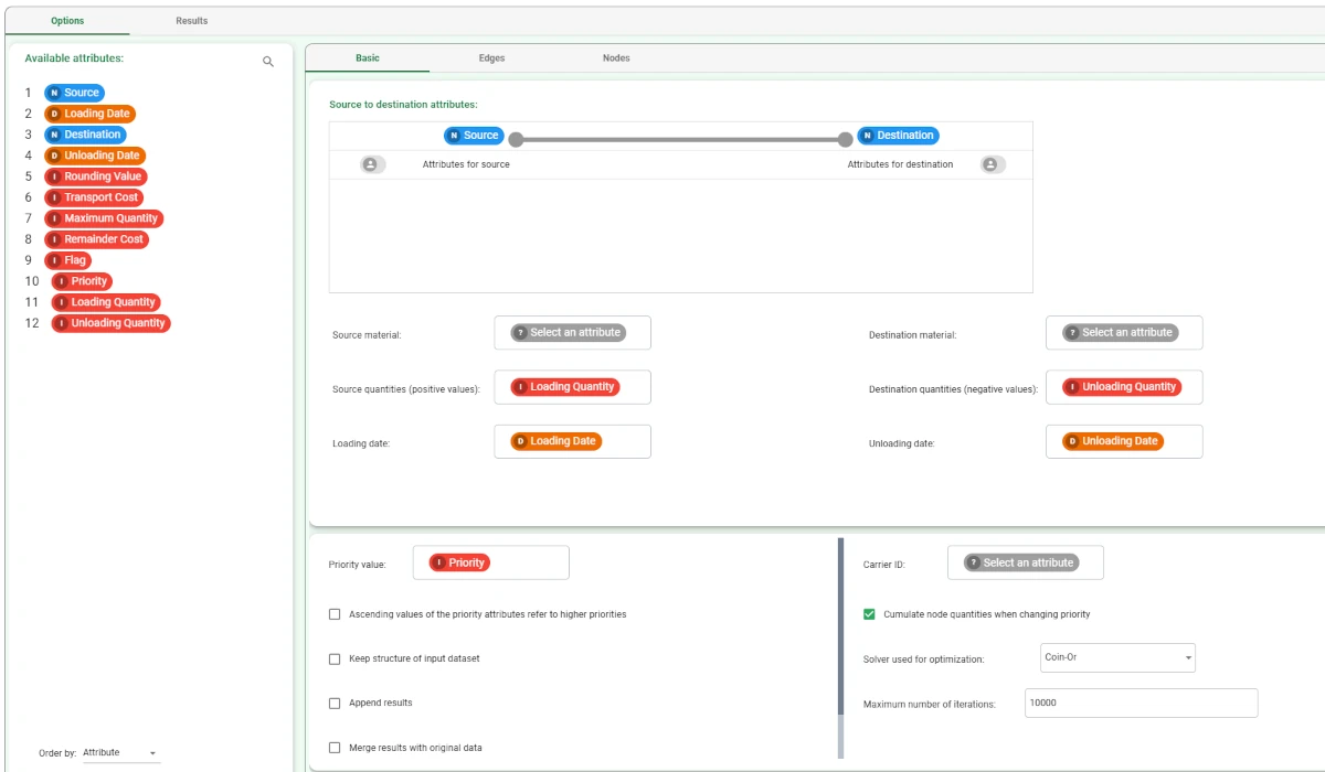
Basic tab

The Basic tab is divided into two areas:

• An attribute drop area, called Source to destination attributes, whose layout is similar to the Matching attributes for joining dataset section in the Join task, where the source and destination attributes will be dropped and linked one to the other. Multiple attributes can be specified there, as long as the source and destination number of attributes are equal. Every source attribute needs to be connected to a destination attribute, so no attribute both in the source and destination lists can be left unpaired.

  The following options are available in this area:

  • Source material: the attribute defining the material at the source. It can be of nominal or integer type.

  • Destination material: the attribute defining the material at the destination. It can be of nominal or integer type.

  • Source quantities: the attribute defining the initial quantity in the source. Its type must be ordered, and its values can both be positive and negative. A positive value indicates the available material which can be moved, while a negative value indicates a demand which must be satisfied.

  • Destination quantities: the attribute defining the required quantity in the destination node. Its type must be ordered, and its values can both be positive and negative. A positive value indicates the quantity available, while a negative value indicates a demand which must be satisfied.

  • Loading date: the attribute defining the date where goods in the source attribute can leave the warehouse and arrive to the destination on the date specified in the Unloading date attribute.

  • Unloading date: the attribute defining the date where goods which have left the source on the Loading date arrive to the destination.

• A customization area, made of the following options:

• Priority value: select the attribute defining the priority of the destinations to which the goods will be sent. Its type must be numeral. The value 1 indicates the highest priority, 2 a priority lower than 1, and so on.

• Ascending values of the priority attributes refer to higher priorities: if selected, a higher value in the Priority value attribute indicates higher priority. (e.g.: if the Priority value 25 has a higher priority than the Priority value 15)

• Keep structure of input dataset: if it is unchecked (default), all the lanes for the priority 1 are included. For the other priorities, only the lanes where goods have actually been moved are included. If the option is selected, the output dataset results are aggregated by lane, while maintaining the original input dataset structure, which affects the output dataset structure, as explained here.

• Append results: if selected, the results of this computation are appended to the dataset, otherwise they replace the results of the previous computations.

• Merge results with original data: if selected, results will be included in the original dataset.

• Put in the output dataset the projected inventory: if selected, a new section containing new rows is added at the end of the dataset. These rows contain the details about the final inventory at each node (seen as destination) and on each considered date (seen as unloading date).

• Carrier ID: select the attribute defining the carrier.

• Cumulate node quantities when changing priority: if selected (default), the node quantities will be cumulated when changing the priority.

• Solver used for optimization: select the solver which will be used for the optimization operation. Possible solvers are:

  • Coin-or: it is a collection of interoperable open source solvers from the repository of open source software maintained by the COIN-OR Foundation. More information can be found in the website.

  • Symphony: it is an open-source generic MILP solver, callable library, and extensible framework for implementing customized solvers for mixed-integer linear programs (MILPs). More information can be found in the website.

  • Naive: it is an optimizer developed by Rulex delivering near-optimal solutions within a remarkably short timeframe.

  • Fast: it is an optimizer developed by Rulex which optimizes the results by prioritizing fast performance over achieving the optimal solution.

• Maximum number of iterations: the maximum number of iterations during computation.

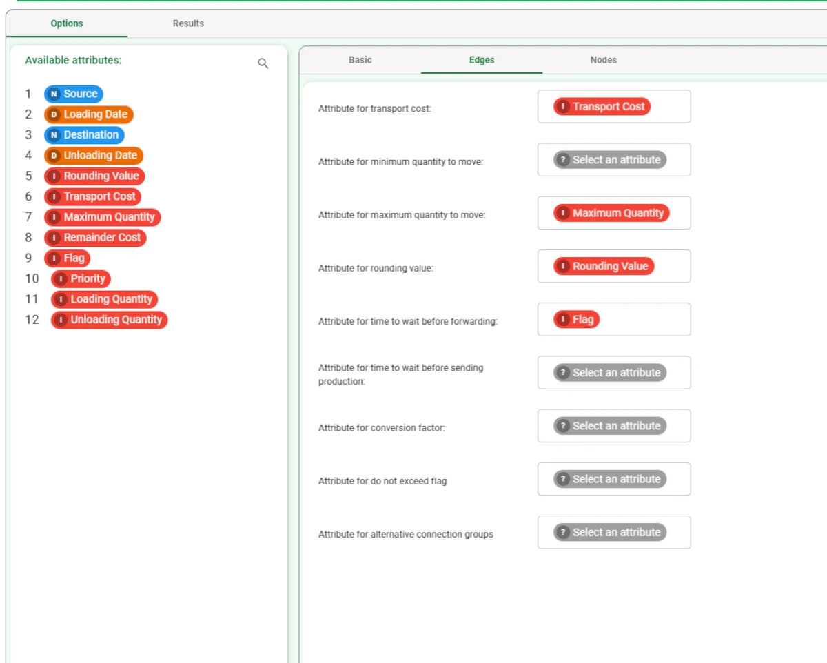
Edges tab

In the Edges tab, you can define the links’ edges. The following options are provided:

• Attribute for transport cost: select the attribute defining the cost of moving a unit of material from the source to the destination.

• Attribute for minimum quantity to move: select the attribute that defines the minimum total number of units which must be moved between the source and the destination at a time. If a quantity lower than the one indicated in this attribute needs to be moved, no goods will be moved.

• Attribute for maximum quantity to move: select the attribute that defines the maximum total number of units which can be moved between the source and the destination at a time.

• Attribute for rounding value: select the attribute that defines the minimum number of units that can be moved at a time. For example, three items may be required, but the items may only be available in blocks of ten.

• Attribute for time to wait before forwarding: select the attribute indicating the waiting time in an intermediate node for the goods to their destination (e.g.: quality control, customs operations).

• Attribute for time to wait before sending production: select the attribute indicating the waiting time in an intermediate node for the goods which are produced or are already stored in the destination node.

• Attribute for conversion factor: select the attribute containing the conversion factor (integer or continuous type), which is a coefficient to convert the current material to another material (e.g., truck, how much space the material occupies in the truck).

• Attribute for do not exceed flag: select the attribute (integer or binary type) defining whether the quantity at the destination can be exceeded or not. If the value of this attribute in the corresponding row is True or has a numeral value which is higher than the corresponding Destination quantities attribute, it means that the Destination quantity quantity is the maximum amount of goods the destination can receive.

• Attribute for alternative connection groups: select the attribute (nominal or integer type) that identifies the lane groups for transporting a specific material from a specific source to a specific destination within given departure/arrival dates. This option is useful when multiple lanes exist for the same material, source, destination group, and based on the optimization process, the task chooses the single lane that best solves the problem.

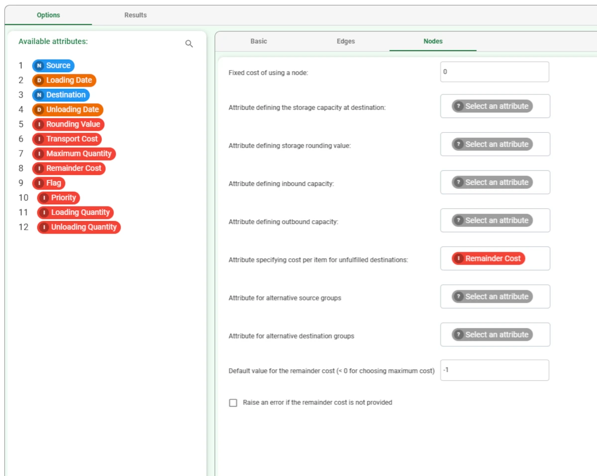
Node tab

In the Nodes tab, you can define the nodes. The following options are provided:

• Fixed cost of using a node: specify the inherent cost of shipping to a node as a quantitative weight to be applied in calculating the best solution.

• Attribute defining the storage capacity at destination: choose the attribute (integer or continuous) that defines the maximum pallet storage capacity of the destination.

• Attribute defining storage rounding value: select the attribute containing the number of materials which are present in a single pallet.

• Attribute defining inbound capacity: select the attribute indicating the maximum number of materials which can be received by the destination node on a given date and time.

• Attribute defining outbound capacity: select the attribute containing the maximum number of materials which can be sent from the source node on a given date and time.

• Attribute specifying cost per item for unfulfilled destinations: select the attribute that defines the cost per unit of not satisfying destination requirements.

• Attribute for alternative source groups: select the attribute (nominal or integer type) that identifies source groups for a specific material at a given date. This option is useful when different source values are present in different rows for the same material, destination, unloading date combinations. For each group, the task will choose only one source.

• Attribute for alternative destination groups: select the attribute (nominal or integer type) that identifies destination groups for a specific material at a given date. This option is useful when different destination values are present in different rows for the same material, source, loading date combinations. For each group, the task will choose only one destination.

• Default value for the remainder cost (<0 for choosing the maximum cost): define the default value used for the remainder cost when the corresponding attribute is not specified or its value is missing. The default value is ‘-1’, meaning that the remainder cost is higher than any transport cost.

• Raise an error if the remainder cost is not provided: if selected, the software raises an error if the remainder cost attribute is not present.

---

The Results tab

In the Results tab, results on computation are displayed.

• In the General Info panel, the following information can be found:

  • the Task Label

  • the Elapsed time

  • the Optimum value of the cost function

---

Input Dataset

The Distribution Planner task accepts only one input dataset. The dataset structure must follow one of two layouts:

• Row layout - each row represents a connection between a source and a destination. The following details are mandatory: source, destination, loading date, unloading date, availability and demand. In other words, each row corresponds to one lane with all its details.

• Zone layout - the dataset is divided into three sections to reduce the total number of rows. It is structured as follows:

  • the first area contains the details on the lanes, so only the attributes indicating the source name, the destination name, the loading date and the unloading date are filled.

  • the second area contains the source description, so only the attributes indicating the source name, the loading date and the source availability (if different from 0) are filled.

  • the third area contains the demand description, so only the attributes indicating the destination name, the unloading date and the demand (if different from 0) are filled.

Using the zone layout avoids generating excessively large datasets, since each lane is described only once. In contrast, the row layout requires each lane to be described separately for every priority.

---

Example

The following example uses the Demand dataset.

• After having imported the dataset, add a Distribution Planner task onto the stage and link it to the import task.

• Open the Distribution Planner task and set the Basic tab options as follows:

  • Drag the Source and the Destination attributes onto the Source to destination attributes drop area, one on each side, and link them.

  • Select the Loading Quantity attribute as the Source quantities attribute.

  • Select the Unloading Quantity attribute as the Destination quantities attribute.

  • Select the Loading Date attribute as the Loading date attribute.

  • Select the Unloading Date attribute as the Unloading date attribute.

  • Select the Priority attribute as the Priority attribute.

  • Select the Cumulate node quantities when changing priority checkbox.

• In the Edges tab, configure the following options:

  • Select the Transport Cost attribute as the Attribute for transport cost.

  • Select Maximum Quantity attribute as the Attribute for maximum quantity to move.

  • Select the Rounding Value attribute as the Attribute for rounding value.

  • Select the Flag attribute as the Attribute for time to wait before forwarding.

• In the Nodes tab, select the Remainder Cost as the Attribute specifying cost per item for unfulfilled destinations.

• Leave all the default settings unchanged.

• Save and compute the task.

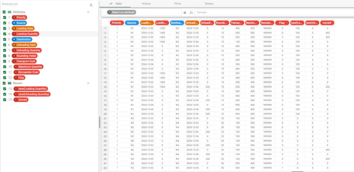
• Right-click on the task and select Take a look, alternatively add a Data Manager task to the flow and link it to the Distribution Planner task.

• This is how the output dataset should look like.

See also

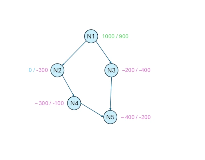
This is a sample of the logic which has been followed by the task with the configuration above. Considering the same date of departure, each node has a demand.

There are five nodes, the N1 is the source node, while the N5 is the destination node.

For each node, two values are indicated: the value on the left has higher priority, while the value on the right has lower priority. Remember that positive values indicate the availability, while negative values indicate the demand.

The difficulty of this optimization problem is that the intermediate nodes, which are N2, N3, N4, are intermediate steps to reach the destination N5, and they have no supply to send to the destination node, even though they are both source and destination nodes.

So, it is necessary that the goods go through these intermediate steps to satisfy the demand of N5.

• Starting to analyze the first priority, we observe that with an initial availability of 1,000 items in N1, the demands of all other nodes can be fully satisfied according to their maximum load requirements. As these demands are 0, 200, 300, and 400 items, respectively. After having subtracted the demand to the availability, 100 goods are still available in the first priority amount, which will be summed to the availability in the second priority, as in the example above we have checked the Cumulate node quantities when changing priority option.

• Analyzing the second priority, which has a starting availability of 1000 (which is 900 in the diagram plus the 100 cumulated from the first priority), we can notice that all the demands can be satisfied as well, having 300, 400, 100, 200 as demand values. If these demands are subtracted to the starting value, the N1 node has 0 availability for both priorities.

The values in the diagram already take into account the cost of moving goods as well as the rounding value and the waiting time.