Auto Regressive
As previously described, Regression tasks contain modelling techniques able to predict a continuous target variable. The Auto Regressive task is highly useful as it forecasts future values over time, mainly based on past behavior.
The task is divided into three tabs:
The Options tab, where users can choose the attribute they will work on and with.
The Models tab, where users can visualize the coefficient values.
The Results tab, where users can visualize a summary of the computation.
The Options tab
The Options tab is divided into two tabs: the Basic tab and the Advanced tab.
In the Basic tab, users will find the following structure:
Available attributes, where users will find the dataset’s attributes. It is always displayed on both Basic and Advanced tabs.
Attributes drop area, where users can drag the chosen attributes.
Customization pane, where users are able to customize different options.
Available attributes
Within this section, users will find a list of all the dataset’s attributes. To search for a specific attribute, use the lens icon at the top right of the panel.
Users also have the option of sorting the attributes according to their preferences. They can choose from a drop-down list of the Order by option:
Attribute
Name
Type
Ignored
Role
Attributes drop area
Within this pane, users can set and configure the following options:
Time series attributes (ORDERED): the ordered attribute which will be used to perform auto regression. Users here can drop the chosen attributes via a Manual list (through a simple operation of dragging and dropping) or via a Filtered list.
Exogenous attributes (ORDERED): additional attributes that need to be considered when performing auto regression predictions. For example, the external temperature could be considered an exogenous attribute when calculating the consumption of energy in heating a house. Users here can drop the chosen attributes via a Manual list (through a simple operation of dragging and dropping) or via a Filtered list.
ID Attributes (NOMINAL): the nominal key attributes that define the rows that will contain the values to be used. Users here can drop the chosen attributes via a Manual list (through a simple operation of dragging and dropping) or via a Filtered list.
Customization pane
Within this pane, users can set and configure the following options:
Interval dimension for time series attributes: the number of previous values to be used in the calculation for the time series attribute.
Interval dimension for exogenous attributes: the number of previous values to be used in the calculation for each exogenous attribute.
Time attribute: users can select a specific time attribute from the drop-down list to specify the temporal variable to be used to set the moving window.
Time lag: the length of each time interval.
Time unit: users can select a specific time unite from the drop-down list. Available values are:
Second(s)
Minute(s)
Hour(s)
Day(s)
Week(s)
Month(s)
Quarter(s)
Year(s)
In the Advanced tab, users can set and configure the following options:
Percentage of constant values for switching to Croston model: when the percentage specified is exceeded the Croston model is used instead of the auto regressive model in the calculation.
Percentage tolerance for switching to Croston model: the tolerance percentage in the range of variation for constant values. When this percentage is not exceeded, the values are considered constant when deciding if the Croston model is to be used or not.
Obsolescence coefficients: users can select the column that contains the obsolescence coefficient to be applied to the time series.
Smoothing function on time series: the function to be used to smooth the values in the time series. Available values are:
Log (transforms the input variables using the log-exponential smoothing technique)
Box-Cox (transforms the input variable using a Box-Cox transformation)
None (no function is used to smooth the input variable)
Interval dimension on time series for rolling mean: if users want to use the rolling mean of past values rather than single values, they need to specify here how many values will be included in each rolling value group. The option specifies the total number of groups used.
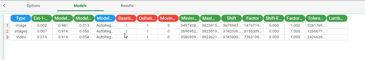
Models tab
Within this tab, users will be able to visualize the coefficient values. Moreover, any periods that have been retrieved and other statistical parameters - such as minimum and maximum - will be displayed.
Results tab
Within this tab, users can visualize a summary of the computation.
This tab is divided into two panes:
General Info
Within this pane, users can find the following information:
Task Label
Elapsed time (sec)
Result Quantities
Within this pane, users can visualize the following option:
Error on data samples
This checkbox is checked by default.
On the right of the above-mentioned checkbox, users, through a drop-down list, will be able to visualize useful information.
Error on data samples:
Train
Test
Valid
Whole
Example
The following example uses the Instagram data dataset.
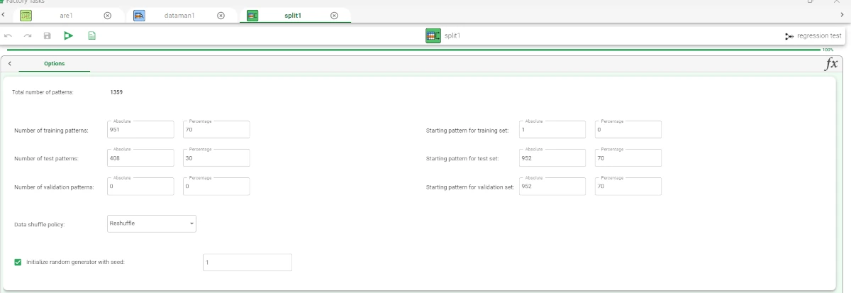
After having imported the dataset via an Import from Text File task, randomly split the dataset into two subsets (test and training set; 30% test and 70% training) with a Split Data task.
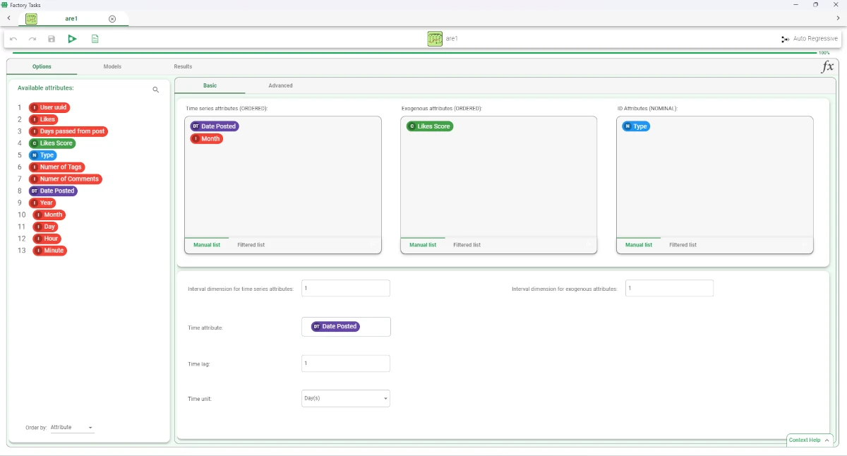
Add an Auto Regressive task and link it to the Split Data task. Open the Auto Regressive task and specify the following parameters:
Time series attributes (ORDERED):
Date Posted
Month
Exogenous attributes (ORDERED):
Likes Score
ID attributes:
Type
Time unit:
Day(s)
After having saved and compute the task, the coefficient values can be visualized in the Models tab.