Statistical functions
Statistical functions perform statistical operations on the selected columns.
They are useful if you need to add the operations performed in the statistics manager directly to your dataset.
The following functions are available:
anovap
The anovap function verify that a certain quantitative variable (dependent variable) keeps the same stochastic distribution against the clusters which have been led by a nominal variable (independent variable).
Hint
- The null hypothesis states that when the independent variable varies, the dependent variables’ distribution doesn’t change, whereas the alternative hypothesis is the consequence of the null hypothesis’ refusal, which means that the dependent variables’ distribution varies when the independent variable changes.
anovap() returns the p value, that is the probability to obtain the worst case compared to the null hypothesis we are verifying. Values above 0.05 (i.e. the conventional value for alpha) state that we can’t reject the null hypothesis, while values below 0.05 state that we need to reject the null hypothesis and consider the alternative one.
Parameters
anovap(column, attclass, group, usemissing)
Parameter |
Description |
|---|---|
column1 |
The continuous attribute used to evaluate the ANOVA p or t value. The column1 parameter is mandatory. |
attclass |
The nominal attribute used to evaluate the ANOVA p or t value. If it is not nominal, it will be cast to nominal upon function’s computation. The attclass parameter is mandatory. |
group |
The attribute used to group results. More than one column can be specified in this parameter, as long as all attributes are enclosed in double brackets. |
usemissing |
A Boolean which indicates whether missing values should be considered or not in the computation of the statistics. The default value, if not otherwise specified, is True. |
Example - anovap(column, attclass)
The following example uses the make single offer tariff order dataset.
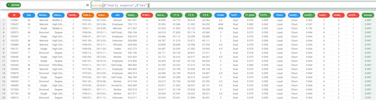
In this example, we want to retrieve the anovap value using the same attributes as in the example above.
The formula to write is:
anovap($"Yearly expense",$"Sex")
Example - anovap(column, attclass, group)
The following example uses the make single offer tariff order dataset.
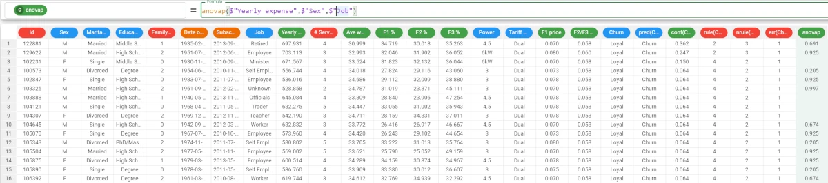
If we want to be more precise with the analysis, we can add the group parameter, as we want our results to be grouped by the Job attribute.
The formula to write is:
anovap($"Yearly expense",$"Sex",$"Job")The results are as follows: * The p value of the Retired people is 0.691; * The p value for the Employees is 0.925, and so on.
As the alpha value is 0.05, we can’t reject the null hypothesis considering the Retired group (i.e. a value of the Job attribute), so the Yearly expense for the males and the females (i.e. the values of the Sex attribute, the independent variable) follows the same stochastic distribution.
anovat
The anovat functions verify that a certain quantitative variable (dependent variable) keeps the same stochastic distribution against the clusters which have been led by a nominal variable (independent variable).
Hint
- The null hypothesis states that when the independent variable varies, the dependent variables’ distribution doesn’t change, whereas the alternative hypothesis is the consequence of the null hypothesis’ refusal, which means that the dependent variables’ distribution varies when the independent variable changes.
anovat() returns the ANOVA test value.
Parameters
anovat(column, attclass, group, usemissing)
Parameter |
Description |
|---|---|
column1 |
The continuous attribute used to evaluate the ANOVA p or t value. The column1 parameter is mandatory. |
attclass |
The nominal attribute used to evaluate the ANOVA p or t value. If it is not nominal, it will be cast to nominal upon function’s computation. The attclass parameter is mandatory. |
group |
The attribute used to group results. More than one column can be specified in this parameter, as long as all attributes are enclosed in double brackets. |
usemissing |
A Boolean which indicates whether missing values should be considered or not in the computation of the statistics. The default value, if not otherwise specified, is True. |
Example - anovat(column, attclass)
The following example uses the make single offer tariff order dataset.
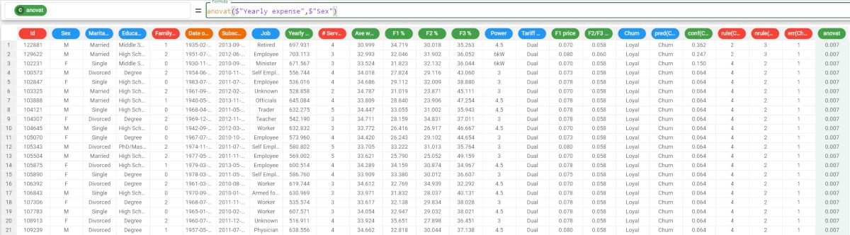
In this example, we want to retrieve the anovat value of the Yearly expense attribute.
The formula to write is:
anovat($"Yearly expense",$"Sex")
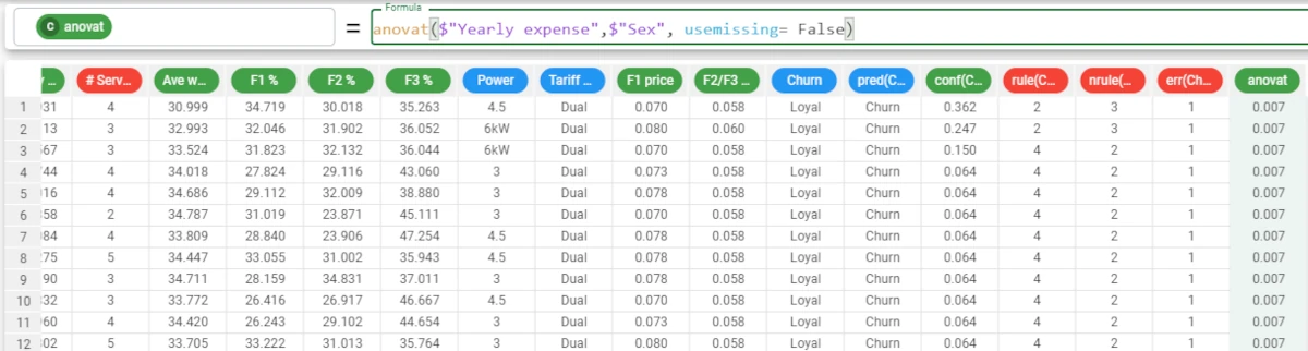
Example - anovat(column, attclass, usemissing=usemissing)
The following example uses the make single offer tariff order dataset.
In this example, we have decided to not include any missing values in the calculations, so we want to set the usemissing parameter to
False.As we have not specified a group parameter, we cannot use the position of the parameter to identify it, so we must use the keyword of the parameter to identify its meaning.
So the consequent formula would be
anovat($"Yearly expense",$"Sex", usemissing = False)
argMax
The argMax functions return the number of the row which contains the maximum value of the selected attribute.
If the maximum value is repeated more than once in the column, the function retrieves only the first row number where the maximum value is found.
See also
The argMax statistic is also available in the Sheets tab of the Data Manager.
Parameters
argMax(column, group)
Parameter |
Description |
|---|---|
column |
The attribute you want to use in the function. Multiple attributes can be specified, as long as they are enclosed in double brackets, i.e. column((column1, column2)). The column parameter is mandatory. |
group |
The attribute by which you want to further group results. |
Example - argMax(column)
The following example uses the Bike Sales dataset.
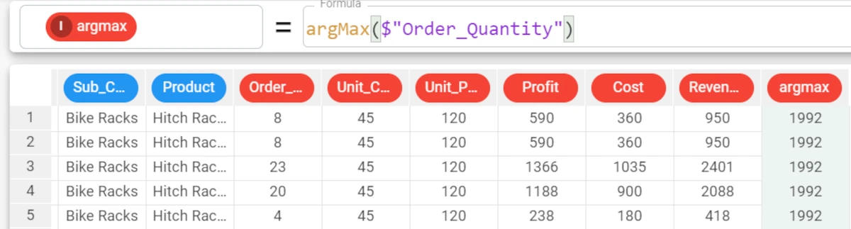
In the example, we want to retrieve the row ID of the maximum value of the Order_Quantity attribute.
Type the formula
argMax($"Order_Quantity")and the attribute will be filled with the row ID of the highest value, which is 1992.
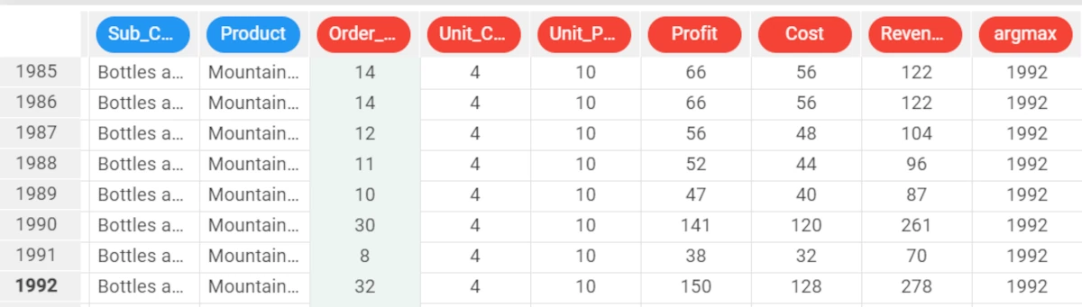
To verify it, go to row 1992. To go to a specific row, right-click on any cell, and select Go to row.
Then, type the row number and click Apply.
The highest value of the Order_Quantity attribute is 32.
We can double-check that the maximum value of the Order_Quantity attribute is 32 by selecting the column and visualizing the basic statistics in the Info panel at the bottom of the screen.
Example - argMax(column, group)
The following example uses the Bike Sales dataset.
If we want to group our results by a certain attribute values, we can specify a group parameter.
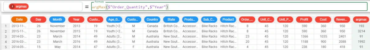
In the example here, we want our results to be grouped by the Year attribute.
The formula will be:
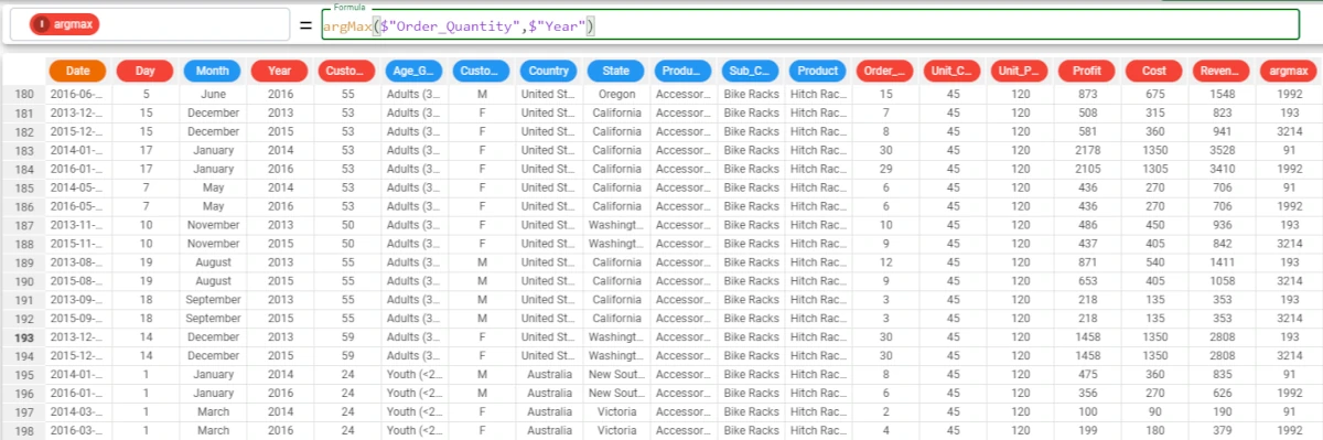
argMax($"Order_Quantity",$"Year")and the attribute will be filled with the row ID of the highest Order Quantity value for each value of the Year attribute.Then, group the results by the Year attribute, in case you need an overview of the argMax for each year. This is an optional operation.
The results are: * For 2013, the maximum value of the Order_Quantity attribute is in row 193; * For 2014, the maximum value of the Order_Quantity attribute is in row 91; * For 2015, the maximum value of the Order_Quantity attribute is in row 3214; * For 2016, the maximum value of the Order_Quantity attribute is in row 1992.
To verify it, go to the specific rows by clicking on any cell and selecting Go to row.
Then, type the row number and click Apply. We want to verify the maximum value for 2013, so we need to go to row 193.
The maximum Order_Quantity value for 2013 is 30.
As you can see in this screenshot, the value 30 is contained also in row 194, but the function returns only the first row ID which contains the maximum of the chosen attribute.
argMin
The argMin functions return the number of the row which contains the minimum value of the selected attribute.
If the minimum value is repeated more than once in the column, the function retrieves only the first row number where the minimum value is found.
See also
The argMin statistic is also available in the Sheets tab of the Data Manager.
Parameters
argMin(column, group)
Parameter |
Description |
|---|---|
column |
The attribute you want to use in the function. Multiple attributes can be specified, as long as they are enclosed in double brackets, i.e. column((column1, column2)). The column parameter is mandatory. |
group |
The attribute by which you want to further group results. |
Example - argMin(column)
The following example uses the Bike Sales dataset.
Now, we want to retrieve the row ID of the lowest value of the Order_Quantity attribute.
Type the formula:
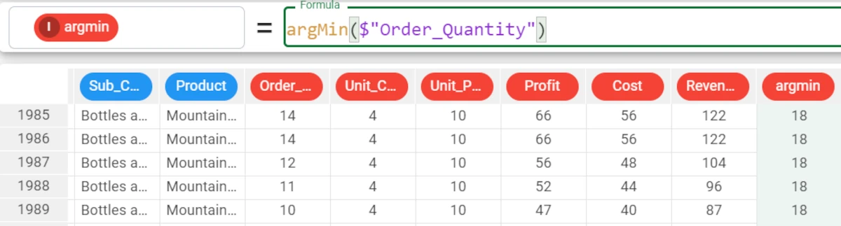
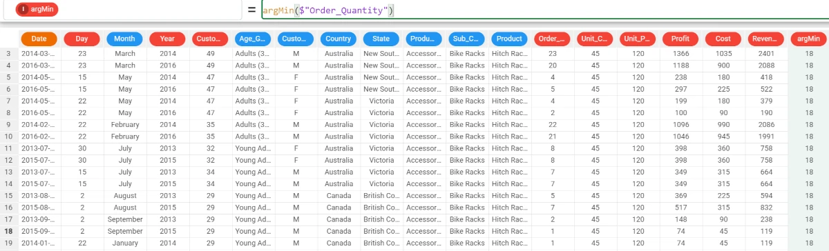
argMin($"Order_Quantity")and the attribute will be filled with the first row ID of the lowest value, that is 18.
To verify it, go to row 18. To go to a specific row, right-click on any cell, row number, column header in the Data Manager and select Go to row.
Then, type the row number and click Apply.
The lowest value of the _Order_quantity_ attribute is 1.
As you can see in this screenshot, the value 1 is contained also in row 19, but the function returns only the first row ID which contains the minimum of the chosen attribute.
chisquare
The chisquare function determine whether there is a correlation between two nominal variables, and evaluates whether the results are sufficiently reliable.
Hint
The null hypothesis states that there is no statistically-significant relationship between two variables in a hypothesis, whereas the alternative hypothesis states the opposite, i.e. that there is a statistically-significant relationship between the variables. * chisquare() determines whether the null hypothesis is true or not. A high value indicates that the variables are independent (so the null hypothesis is true), a low value indicates the opposite (so the alternative hypothesis is true).
See also
The chisquare statistic is also available in the Sheets tab of the Data Manager. In the Sheets tab, the chisquare results are graphically displayed in a contingency table, which shows the frequency distribution of the values of the selected attributes.
Parameters
chisquare(column1, column2, group, usemissing)
Parameter |
Description |
|---|---|
column1 |
The first nominal attribute you want to use in the function. If it is not nominal, it will be cast to nominal upon function’s computation. The column1 parameter is mandatory. |
column2 |
The second nominal attribute you want to use in the function. If it is not nominal, it will be cast to nominal upon function’s computation. The column2 parameter is mandatory. |
group |
The attribute used to group results. If the column1 and column2 parameters are already a list, the group parameter is ignored. |
usemissing |
A Boolean which indicates whether missing values should be considered or not in the computation of the statistics. The default value, if not otherwise specified, is True. |
Example - chisquare(column1, column2)
The following example uses the HR employee attrition dataset.
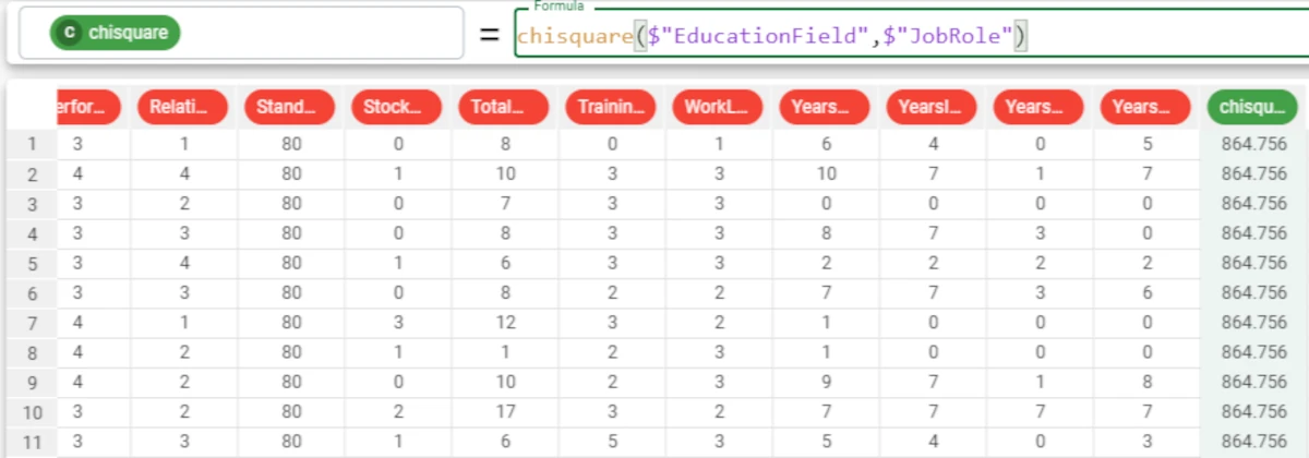
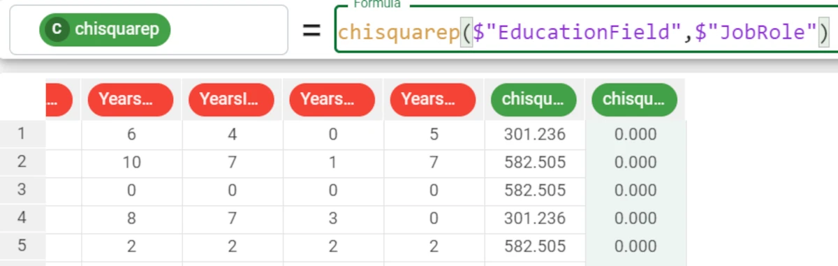
In the example here, we want to retrieve the chisquare statistic of the Education Field and Job Role attributes, to understand if there is a correlation between education and job roles for the samples in the dataset. We write the formula
chisquare($"EducationField",$"JobRole")and the attribute will be filled with the chisquare value, which is 864.756.
Example - chisquare(column1, column2, group)
The following example uses the HR employee attrition dataset.
If we want our results to be grouped by another attribute, we simply add the attribute name to the formula.
So our formula will be:
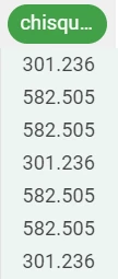
chisquare($"EducationField",$"JobRole",$"Gender")As we can see, the results have changed: * The chisquare value for the female gender is 301.236; * The chisquare value for the male gender is 582.505.
chisquarep
The chisquarep function determine whether there is a correlation between two nominal variables, and evaluates whether the results are sufficiently reliable.
Hint
The null hypothesis states that there is no statistically-significant relationship between two variables in a hypothesis, whereas the alternative hypothesis states the opposite, i.e. that there is a statistically-significant relationship between the variables.
chisquarep() compares the null hypothesis, which assumes the variables are totally independent, to the results obtained by analyzing the data (the alternative hypothesis), to evaluate the reliability of the correlation. The result is a coefficient, which indicates the lowest level of significance at which the null hypothesis of the coefficient would be rejected. Values can range between 0 and 1, where low values below 0.05 indicate that there may effectively be a correlation between the variables, whereas higher values indicate that the results are probably due simply to chance, and cannot consequently be considered reliable. This value is particularly important to consider when the dataset has a limited number of samples.
See also
The chisquare statistic is also available in the Sheets tab of the Data Manager.
In the Sheets tab, the chisquare results are graphically displayed in a contingency table, which shows the frequency distribution of the values of the selected attributes.
Parameters
chisquarep(column1, column2, group, usemissing)
Parameter |
Description |
|---|---|
column1 |
The first nominal attribute you want to use in the function. If it is not nominal, it will be cast to nominal upon function’s computation. The column1 parameter is mandatory. |
column2 |
The second nominal attribute you want to use in the function. If it is not nominal, it will be cast to nominal upon function’s computation. The column2 parameter is mandatory. |
group |
The attribute used to group results. If the column1 and column2 parameters are already a list, the group parameter is ignored. |
usemissing |
A Boolean which indicates whether missing values should be considered or not in the computation of the statistics. The default value, if not otherwise specified, is True. |
Example - chisquarep(column1, column2)
The following example uses the HR employee attrition dataset.
In this example we would like to check the reliability of a retrieved chisquare.
We write the formula:
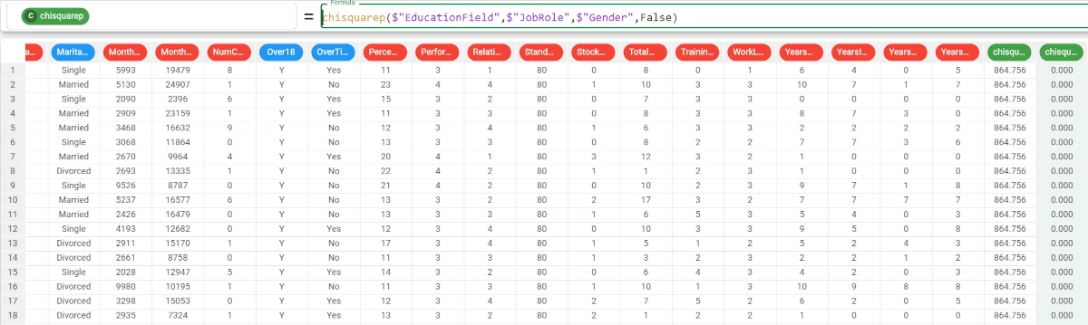
chisquarep($"EducationField",$"JobRole")and the attribute will be filled with value of the p coefficient, which is 0.
Example - chisquarep(column1, column2, group)
The following example uses the HR employee attrition dataset.
If we want our results to be grouped by another attribute, we simply add the attribute name to the formula.
In this case, we also do not want to consider any missing values in the calculations, so we set the usemissing parameter to False.
So our formula will be:
chisquarep($"EducationField",$"JobRole",$"Gender",False)
cohenk
The cohenk function applies the Cohen kappa’s coefficient to compare values. It is commonly used to compare real and predicted values to evaluate model performance, considering the probability of agreement by pure chance.
Hint
Its resulting value can range from 0 to 1:
0 corresponds to a totally random correspondence.
1 indicates complete correspondence between the values, and consequently indicative the best performance.
The value can also be negative, and it indicates a poor performance.
See also
Cohen Kappa’s coefficient is also available in the Sheets tab of the Data Manager.
Parameters
cohenk(column1, column2, group, usemissing)
Parameter |
Description |
|---|---|
column1 |
The first attribute you want to use in the function. The column1 parameter is mandatory. |
column2 |
The second attribute you want to use in the function. The column2 parameter is mandatory. |
group |
The attribute by which you want to further group results. |
usemissing |
A Boolean which indicates whether missing values should be considered or not in the computation of the statistics. The default value, if not otherwise specified, is True. |
Example - cohenk(column1, column2)
The following example uses the Bike Sales dataset.
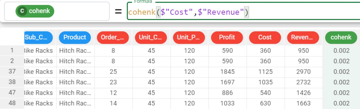
In the example here, we want to retrieve the Cohen K coefficient from the relationship between the Cost and the Revenue.
We type the following formula:
cohenk($"Cost",$"Revenue")
Example - cohenk(column1, column2, group)
The following example uses the Bike Sales dataset.
If we want to focus our analysis on certain groups, we simply need to add the group parameter.
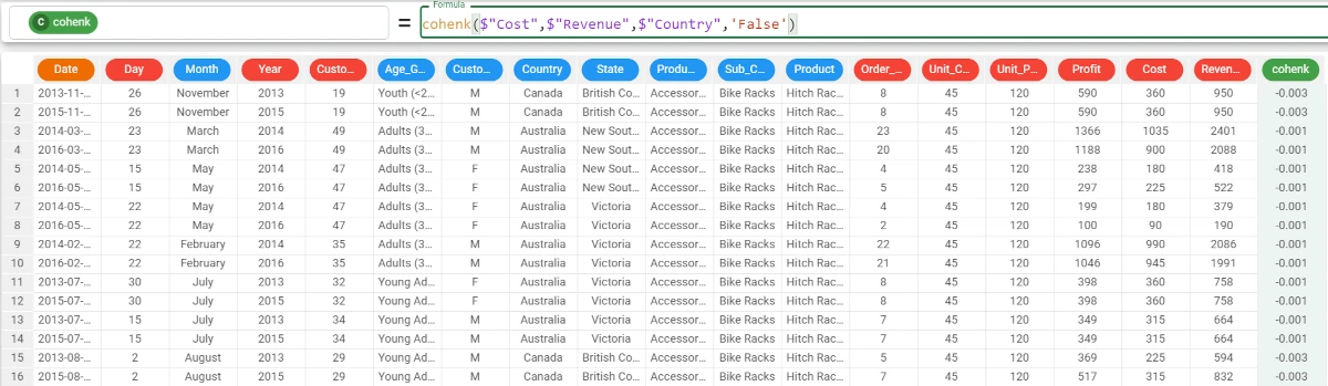
For example, we want to calculate the Cohen K coefficient between the Cost and Revenue attributes, grouping our results by the Country attribute, and we want the string
Noneto be displayed if in any of the first two columns there are some missing values.The formula to write will be:
cohenk($"Cost",$"Revenue",$"Country",'False')The results are: * The Cohen K between Cost and Revenue is -0.003 for Canada; * The Cohen K between Cost and Revenue is -0.001 for Australia and so on.
count
The count function returns the number of times each distinct value is present in an attribute.
In its most simple form, count(), it can also be used to simply count the number of overall values in an attribute.
See also
The count function is available also by dragging the attribute onto the Apply tab of the Query Manager, and selecting Count.
Parameters
count(group)
Parameter |
Description |
|---|---|
group |
The attribute by which you want to group results. A list of attributes can also be provided in the column parameter, as long as they are enclosed in double brackets, i.e. |
Example - count()
The following example uses the Bike Sales dataset.
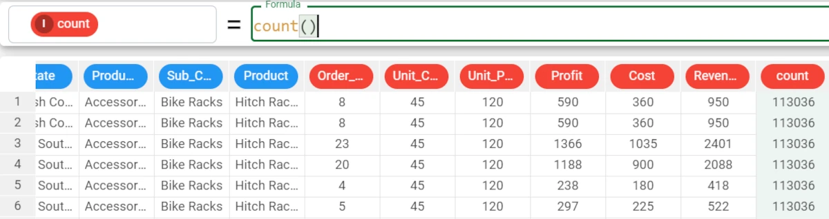
In the example, we want to fill the count attribute with the number of overall values in the attribute. We simply write the formula
count()and the attribute will be filled with the number of values, which in this example is113036.
Example - count(group)
The following example uses the Bike Sales dataset.
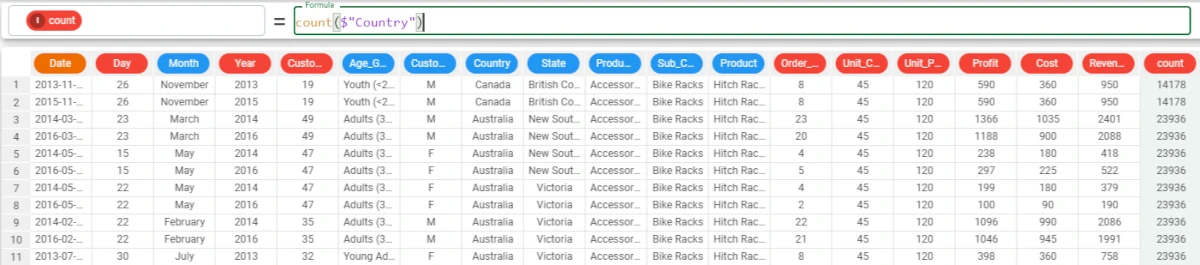
If we want to count the number times distinct values are present in the Country attribute, enter Country in the column parameter.
The formula to write will be:
count($"Country")The results show us that Canada is present in the Country attribute 14178 times, while Australia is present 23936 times, and so on.
Example - count((group1, group2))
The following example uses the Bike Sales dataset.
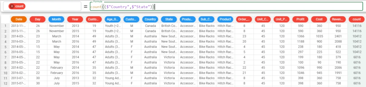
If we want to group the Country results by a State, we can enter both attributes as a list in the column parameter.
The formula to write will be:
count(($"Country", $"State"))The results can be read as follows: * The number of times in the dataset where the Country attribute is Australia and the State attribute is New South Wales is 10412; * The number of times in the dataset that the Country attribute is Australia and the State attribute is Victoria is 6016.
countIf
The countIf function number of times a distinct value, which meets a specified condition, is present in an attribute.
Parameters
countIf(condition,group)
Parameter |
Description |
|---|---|
condition |
The condition that must be met for the value to be counted. The condition parameter is mandatory. |
group |
The attribute by which you want to further group results. |
Example - countIf(condition)
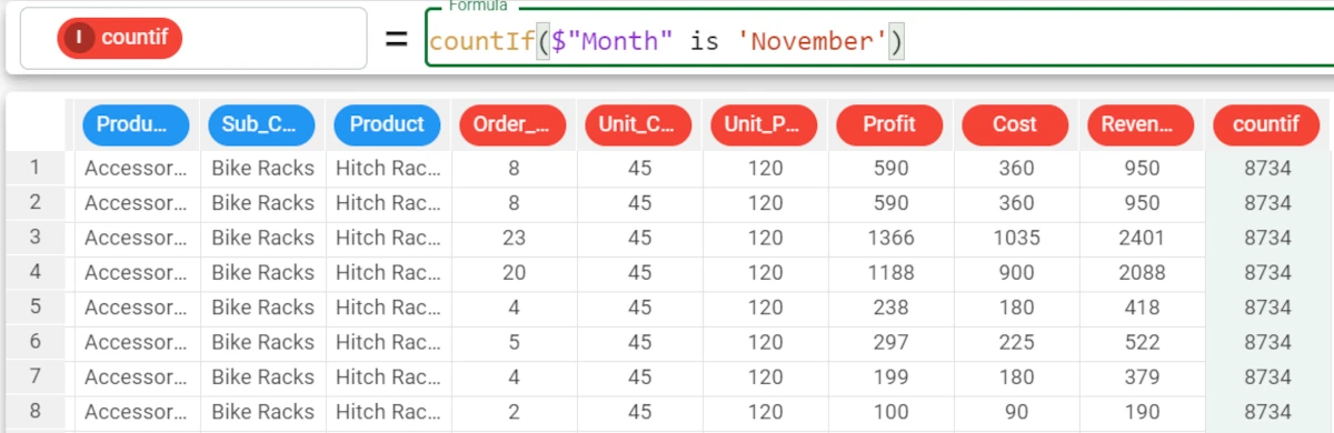
In the example we want to count the number of times the value in the Month attribute is November.
We write the following formula in the formula bar:
countIf($"Month" is $"November")Only the values which satisfy the conditions will be counted. In the Month attribute, the value is November in 8734 rows.
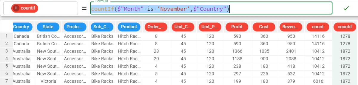
Example - countIf(condition, group)
If we want to group our results, we just need to add a group parameter.
In this example, we want to group our results by the Country attribute values, so we type the formula:
countIf($"Month" is $"November", $"Country")The results are: * In 1278 rows the value of Month is November and the value of Country is Canada; * In 1872 rows the value of Month is November and the value of Country is Australia and so on.
covariance
Covariance is a measure of how changes in one variable are associated with changes in a second variable.
Although it measures the relationship between two variables, it is an absolute measure, not a normalized one, so giving them a quantitative meaning is very difficult. Its corresponding normalized measure is the correlation.
A positive value indicates a positive covariance, while
A negative value indicates a negative covariance.
Parameters
covariance(column1, column2, group)
Parameter |
Description |
|---|---|
column1 |
The first attribute you want to use in the function. The column1 parameter is mandatory. |
column2 |
The second attribute you want to use in the function. The column2 parameter is mandatory. |
group |
The attribute by which you want to further group results. |
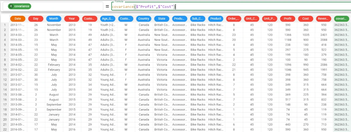
Example - covariance(column1, column2)
The following example uses the Bike Sales dataset.
In this example, we want to retrieve the covariance between the profit and cost attributes.
We type the following formula:
covariance($"Profit",$"Cost")
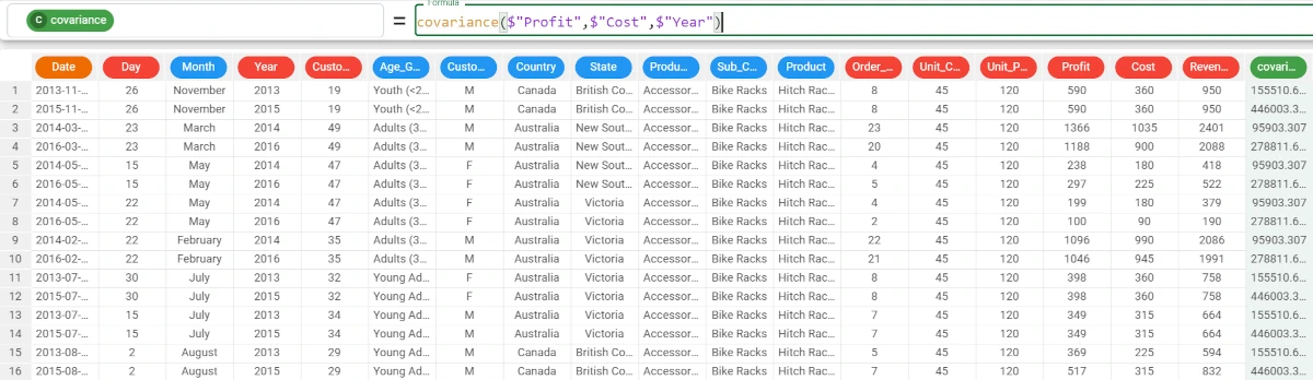
Example - covariance(column1, column2, group)
The following example uses the Bike Sales dataset.
We want to go further with the analysis, and group our results. In this case, we want to group our values by the Year attribute.
The formula will be:
covariance($"Profit",$"Cost",$"Year")The results can be read as follows: * For 2013, the covariance between the Profit and the Cost is 155510.629; * For 2015, the covariance between the Profit and the Cost is 446003.342 and so on. In this example, the covariance between the values is positive, so it displays that, as the Profit value increases, the Cost value tends to increase and vice versa.
cumMax
The cumMax function returns the cumulative maximum of the column, which is the greatest value between the current value of the column and the previous values of the same column, evaluated within groups defined by the group parameter if required.
This function divides the column into rows and compares the values one by one: this means that, if our column is made up of 10 records, the functions will compare row 1, then row 1 and 2, then row 1; 2; 3, then row 1; 2; 3; 4, and so on.
Parameters
cumMax(column, group)
Parameter |
Description |
|---|---|
column |
It identifies the column to which you want to apply the formula. The column parameter is mandatory. |
group |
It allows you to group the results by a certain column. |
Example - cumMax(column)
The following example uses the Bike Sales dataset.
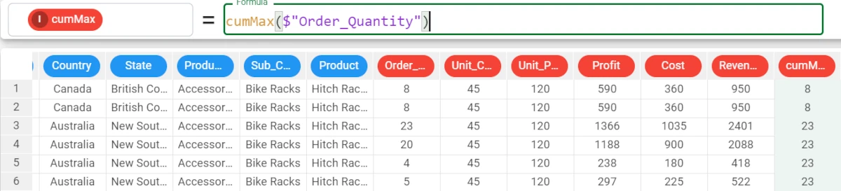
In the example here, we want to fill the cumMax attribute with the cumulative maximum of the Order_Quantity attribute.
The formula to write is:
cumMax($"Order_Quantity")
Example - cumMax(column, group)
The following example uses the Bike Sales dataset.
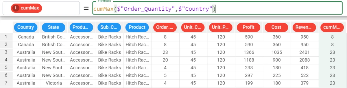
Moving on with our data analysis, we want our cumulative maximum to be grouped by the Country attribute, so our formula will become:
cumMax($"Order_Quantity",$"Country")
cumMin
The cumMin function returns the cumulative minimum of the column, which is the lowest value between the current value of the column and the previous values of the same column, evaluated within groups defined by the group parameter if required.
This function divides the column into rows and compares the values one by one: this means that, if our column is made up of 10 records, the functions will compare row 1, then row 1 and 2, then row 1; 2; 3, then row 1; 2; 3; 4, and so on.
Parameters
cumMin(column, group)
Parameter |
Description |
|---|---|
column |
It identifies the column to which you want to apply the formula. The column parameter is mandatory. |
group |
It allows you to group the results by a certain column. |
Example - cumMin(column)
The following example uses the Bike Sales dataset.
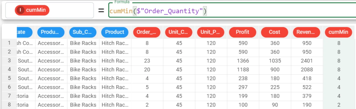
In the example here, we want to fill the cumMin attribute with the cumulative minimum of the Order_Quantity attribute.
The formula to write is:
cumMin($"Order_Quantity")
Example - cumMin(column, group)
The following example uses the Bike Sales dataset.
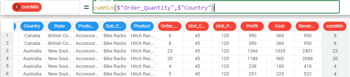
Moving on with our data analysis, we want our cumulative minimum to be grouped by the Country attribute, so our formula will become:
cumMin($"Order_Quantity",$"Country")
distinct
The distinct function returns the number of distinct values of the column, evaluated within groups defined by the group parameter if required.
You can use this function in case you need to fill an attribute with the number of distinct values of another one.
See also
It is possible to visualize the number of distinct values of nominal attributes also by selecting the attribute and reading the result in the Info row bar of the Data Manager task.
Parameters
distinct(column, group,usemissing)
Parameter |
Description |
|---|---|
column |
It identifies the column to which you want to apply the formula. The column parameter is mandatory. |
group |
It allows you to group the results by a certain column. |
usemissing |
Flag used to define if missing values have to be considered or not in distinct values. Default is False. |
Example - distinct(column)
The following example uses the HR employee attrition dataset.
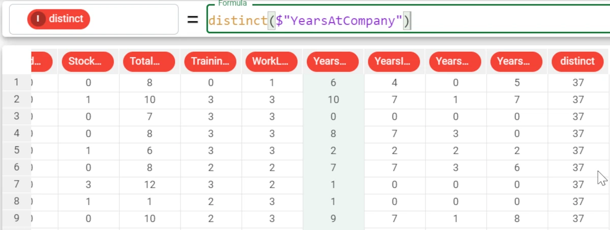
In this example, we want to count the number of distinct values of the YearsAtCompany attribute.
We write the following formula:
distinct($"YearsAtCompany").The number of distinct values for the YearsAtCompany attribute is 37.
Example - distinct(column, group)
The following example uses the HR employee attrition dataset.
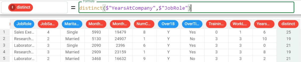
We want to group our results by the JobRole attribute.
So we add to the formula the group parameter, and the formula will be:
distinct($"YearsAtCompany", $"JobRole").- The results will be:
For the Sales Executive role, there are 25 distinct values for YearsAtCompany.
For the Research Scientist role, there are 19 distinct values for YearsAtCompany.
entropy
The entropy function indicates a variable’s unpredictability. The higher the value, the higher the unpredictability.
It returns the entropy of the column, evaluated within groups defined by the group parameter if required.
Hint
- The entropy value is included between 0 and 1, where:
0 indicates low unpredictability, and
+1 indicates high unpredictability.
See also
Parameters
entropy(column, group, usemissing)
Parameter |
Description |
|---|---|
column |
It identifies the column to which you want to apply the formula. The column parameter is mandatory. |
group |
It allows you to group the results by a certain column. |
usemissing |
A Boolean which indicates whether missing values should be considered or not in the computation of the statistics. The default value, if not otherwise specified, is True. |
Example - entropy(column)
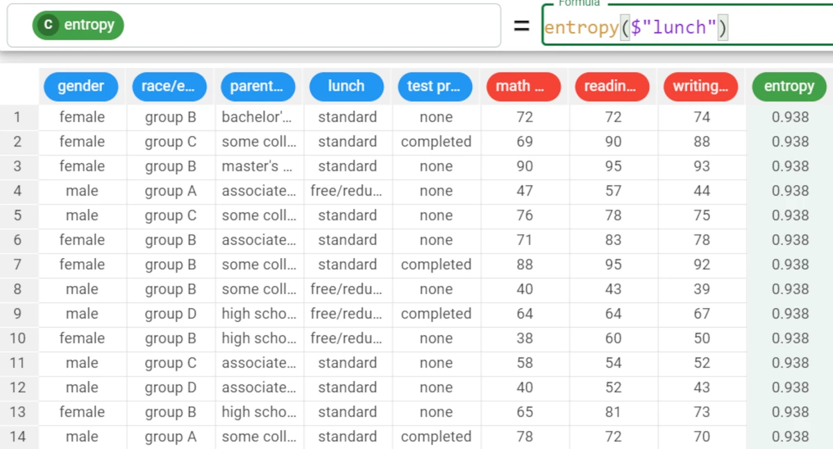
The following example uses the Students Performance dataset.
In the example here, we want to retrieve the Entropy of the lunch attribute’s values.
Write the following formula:
entropy($"lunch").The Entropy value for the lunch attribute is 0.938.
Example - entropy(column, group)
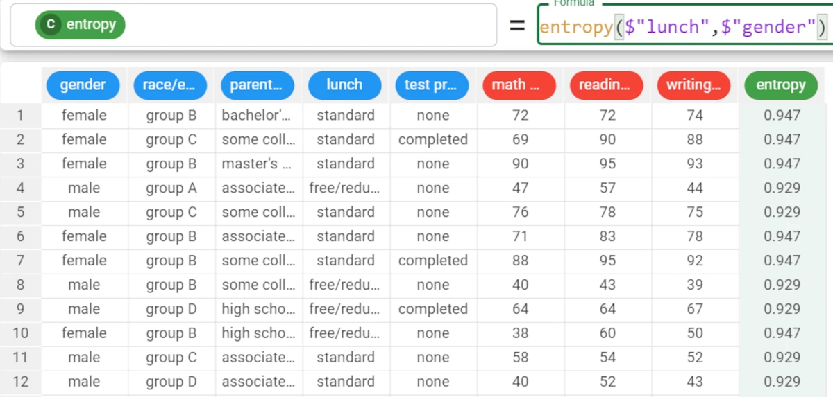
If we want to be more precise with our analysis, we can add the group parameter.
For example, we want to group the results of our entropy by the gender attribute.
Write the following formula:
entropy($"lunch",$"gender").The results will be: * For the female value, the entropy of the lunch attribute is 0.947. * For the male value, the entropy of the lunch attribute is 0.929.
fact
The fact function returns the factorial of the values of the column.
The factorial of a non-negative integer number n is the product of all positive integer values equal or less than the n value.
Parameters
fact(column)
Parameter |
Description |
|---|---|
column |
It identifies the column to which you want to apply the formula. Its type must be integer. If it is not integer, an attempt to convert the attribute to integer is made upon function’s computation. The column parameter is mandatory. |
Example - fact(column)
The following example uses the Bike Sales dataset.
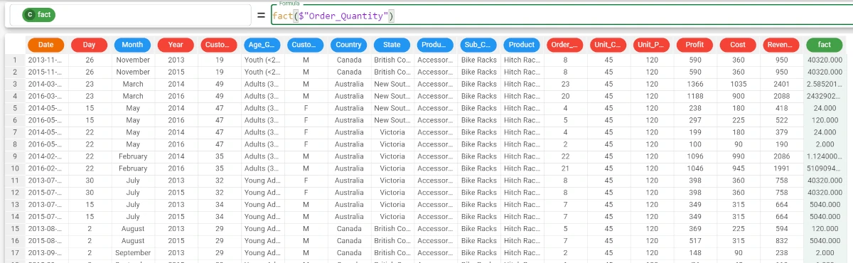
In the example here, we want to retrieve the factorial of the values of the _Order_Quantity_ attribute.
We type the following formula:
fact($"Order_Quantity")
gini
The gini function returns the Gini index of the column, evaluated within groups defined by the group parameter if required.
The Gini index is a measure of statistical dispersion.
Hint
- The Gini index is included between 0 and +1, where:
0 indicates perfect equality between values, and
+1 indicates maximum inequality between values.
See also
The Gini statistic is also available in the Sheets tab of the Data Manager.
Parameters
gini(column, group, usemissing)
Parameter |
Description |
|---|---|
column |
It identifies the column to which you want to apply the formula. The column parameter is mandatory. |
group |
It allows you to group the results by a certain column. |
usemissing |
A Boolean which indicates whether missing values should be considered or not in the computation of the statistics. The default value, if not otherwise specified, is True. |
Example - gini(column)
The following example uses the Adult dataset.
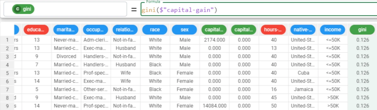
In the example here, we want to calculate the Gini index of the _Capital_Gain_ attribute.
The formula to write is:
gini($"capital-gain")
Example - gini(column, group)
The following example uses the Adult dataset.
If we want to be more precise with our analysis, we can add the group parameter.
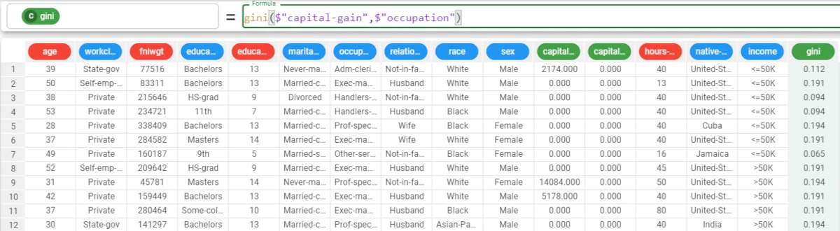
In the example here, we want to group our results by the occupation attribute.
So, the formula to write will be:
gini($"capital-gain",$"occupation").The results are as follows: * The Gini index for Adm-clericals is 0.112; * The Gini index for Exec-managerial is 0.191; * The Gini index for Handlers-cleaners is 0.094, and so on for all the other values of the occupation attribute.
inIqr
The interquartile function isolates outliers: for each data observation, it identifies whether it is in the interquartile deviation or not.
It returns the column with a binary True/False value according to the interquartile range.
The coefficient (coeff) value is 1.5 by default. If another coefficient is needed, you can write it in the formula.
If the coefficient is:
<1, it is considered very restrictive.
>1, it is considered less restrictive.
If $”att” is in [Q1-coeff*(Q3-Q1), Q3+coeff*(Q3-Q1)] (where Q1 and Q3 are the first and the third quartiles, respectively, and coeff is a parameter fixed by the user), inIqr returns True, otherwise it returns False.
See also
The interquartile function is available also in the Sheets tab of the Data Manager.
Parameters
inIqr(column, coeff)
Parameter |
Description |
|---|---|
column |
It identifies the column to which you want to apply the formula. The column parameter is mandatory. |
coeff |
it is a factor fixed by the user to have a more restrictive or a less restrictive result. |
Example - inIqr(column)
The following example uses the Bike Sales dataset.
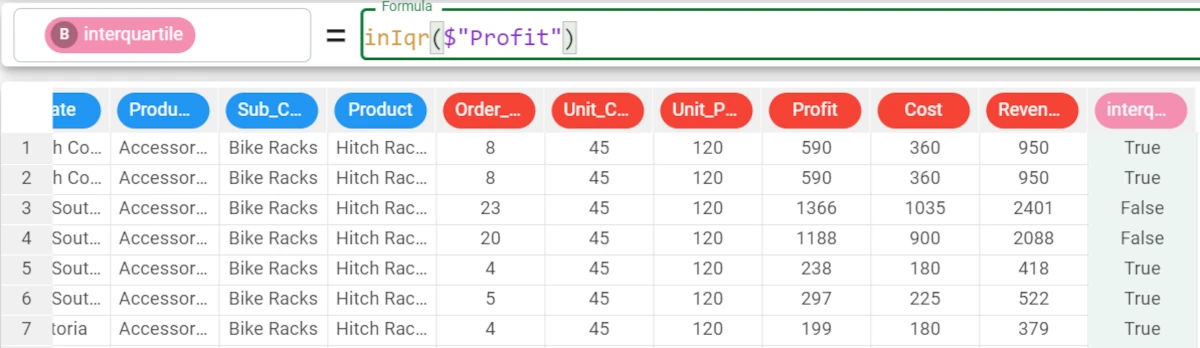
In the example here, we want to retrieve the interquartile of the Profit attribute.
We write the following formula:
inIqr($"Profit").The formula returns
Truewhen the value is an outlier, otherwise aFalseis returned. By default, the coefficient is 1.5.
Example - inIqr(column, coeff)
The following example uses the Bike Sales dataset.
If we want to apply a different coefficient, we only need to specify it in the formula.
In the example here, we want it to be 0.5, so we write:
inIqr($"Profit",0.5).The results have changed, according to the new coefficient.

max
The max function is intended to retrieve the maximum value of an attribute.
The max function retrieves the maximum value of an attribute, eventually grouped, or if a list of attributes is provided in the column parameter it compares the various attributes retrieving the maximum value between them.
See also
The maximum (max) function only is available also by:
Selecting the column in the Data tab and finding the maximum in the Info row bar (for not nominal-like or date-like attributes only).
Dragging the attribute in the Apply‘s query panel.
Selecting the function in the Sheets.
Parameters
max(column, group)
Parameter |
Description |
column |
It identifies the column to which you want to apply the formula. The column parameter is mandatory. |
group |
It allows you to group the results by a certain column. |
Example - max(column)
The following example uses the Students Performance dataset.
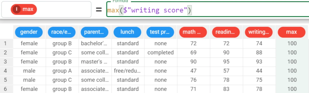
In the example here, we want to fill the max attribute with the maximum of the writing score attribute.
We type the following formula:
max($"writing score")and the function returns the highest value for the writing score.
Example - max(column, group)
The following example uses the Students Performance dataset.
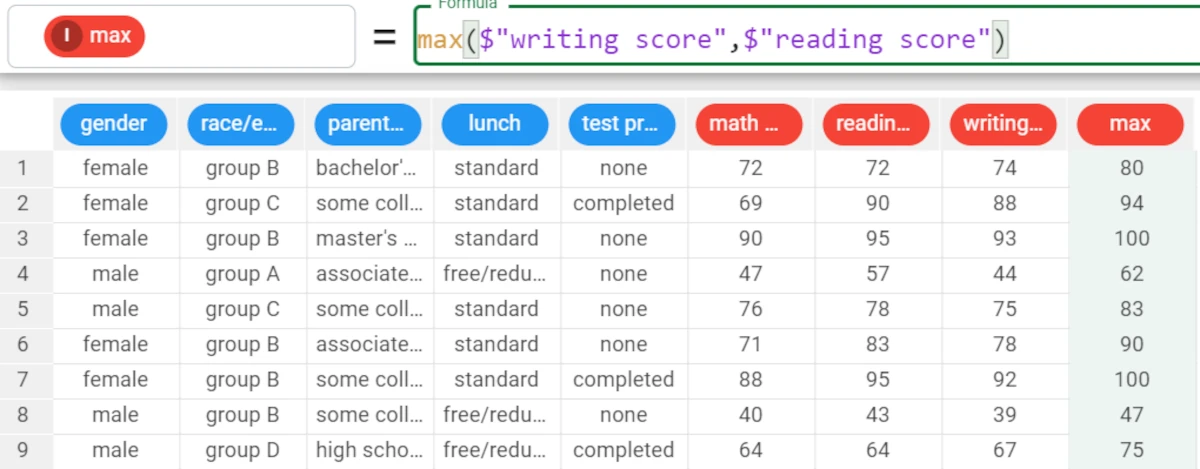
If we want to group our results by their reading score, the formula will be:
max($"writing score",$"reading score")and the function returns the highest value for the writing score, grouped by the reading score.So the results will be: * The maximum writing score value associated with the 72 reading score is 80. * The maximum writing score value associated with the 90 reading score is 94.
Example - max((column1, column2))
The following example uses the Students Performance dataset.
In the example here, we want to compare the writing score and the reading score, and we want to retrieve the highest values between them.
We write the following formula:
max(($"writing score",$"reading score")).The results will be: * In row 1, the maximum value between the writing score value (74) and the reading score value (72) is 74. * In row 2, the maximum value between the writing score value (88) and the reading score value (90) is 90 and so on.
max2
Danger
This function is deprecated for comparing attributes: use instead max((column1, column2)). This function is still useful to compare scalar values between them or scalar values with attributes.
The max2 function compares two elements and retrieves the maximum value between them.
Parameters
max2(elem1, elem2)
Parameter |
Description |
|---|---|
elem1 |
It identifies the element to which you want to apply the formula. The elem1 parameter is mandatory. |
elem2 |
It identifies the element to which you want to apply the formula. The elem2 parameter is mandatory. |
Example - max2(elem1, elem2)
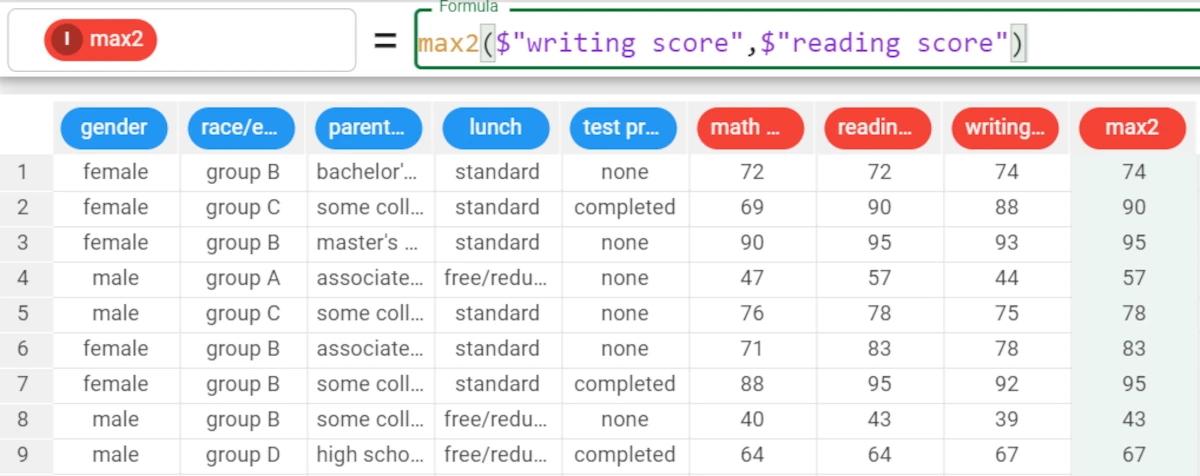
In this example we want to compare the value
Truewith the value2We then write the formula
max2(True, 2)The result will be
2in all the rows sinceTrueis automatically converted in the number1.
maxyoudencut
The maxyoudencut function returns the value which maximizes the youden index of the ROC curve defined by column1 and by the class attclass.
The default value for the class attribute (if more than two values are present) can be specified as the optional parameter defclass.
The computation can be performed according to the groups defined in the group parameter, if required.
Parameters
maxyoudencut(column, attclass, defclass, group, weights)
Parameter |
Description |
|---|---|
column |
It identifies the column to which you want to apply the formula. Its type must be numeral or nominal. The column parameter is mandatory. |
attclass |
It identifies the column to which you want to apply the formula. It must be a nominal attribute. If it is not nominal, it will be cast to nominal upon function’s computation. The attclass parameter is mandatory. |
defclass |
It is the default value for the class attribute. |
group |
The attribute used to group results. Multiple attributes can be specified, as long as they are enclosed in double brackets. |
weights |
It defines the importance of a certain attribute. |
Example - maxyoudencut(column, attclass)
The following example uses the Bike Sales dataset.
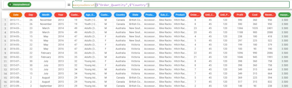
In the example here, we want to calculate the maxyoudencut of the Order_Quantity attribute with the Country target.
The formula to write is:
maxyoudencut($"Order_Quantity",$"Country")
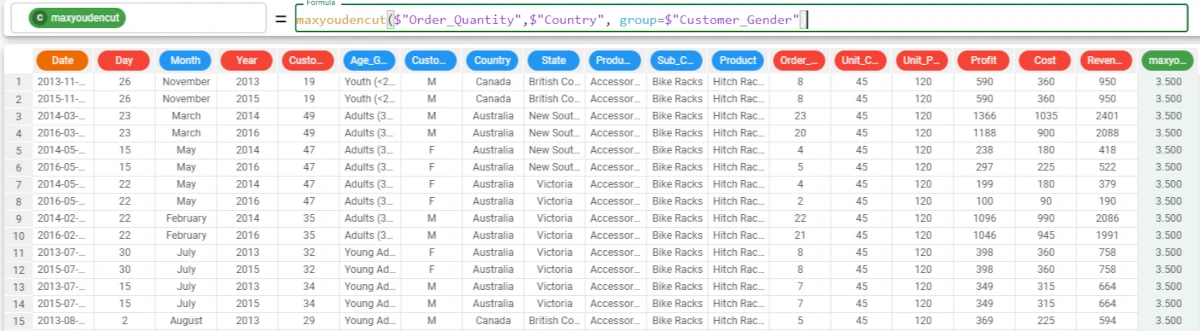
Example - maxyoudencut(column, attclass, group=group)
The following example uses the Bike Sales dataset.
If we want to group our results, we can add the group parameter, that, if the defclass is not defined, must be written as
group=$"att".We want to group our results by the Customer_Gender attribute, so the formula becomes:
maxyoudencut($"Order_Quantity",$"Country",group=$"Customer_Gender").In this case, the results don’t change.
mean
The mean function displays the average attribute value calculated mathematically. It is the sum of the values divided by the number of values. (E.g.: the mean between 2; 3; 10 is 5).
See also
The mean is available also by:
Selecting the column in the Data tab and finding the minimum in the Info row bar.
Dragging the attribute in the Apply area of the Data Manager’s query panel.
Selecting the function in the Sheets tab of the Data Manager.
Parameters
mean(column, group)
Parameter |
Description |
|---|---|
column |
It identifies the column to which you want to apply the formula. The column parameter is mandatory. |
group |
It allows you to group the results by a certain column. |
Example - mean(column)
The following example uses the Students Performance dataset.
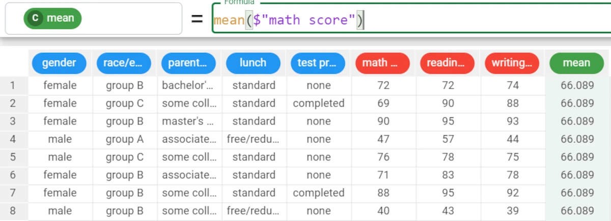
In the example here, we want to retrieve the mean of the math score attribute.
We write the following formula:
mean($"math score").So, the mean of the math score attribute is 66.089.
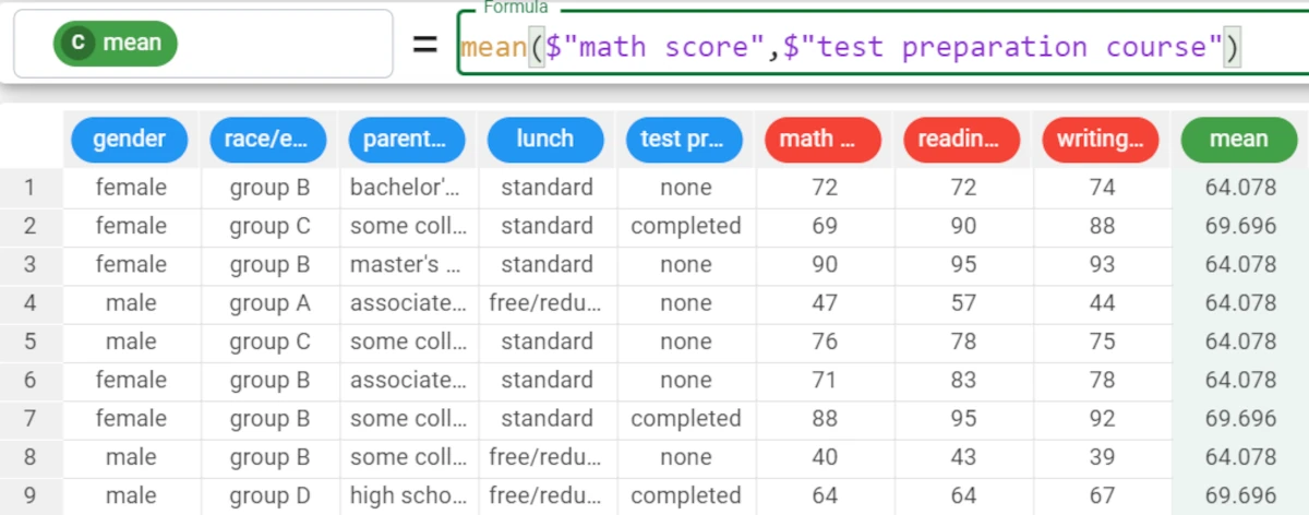
Example - mean(column, group)
The following example uses the Students Performance dataset.
We also want to group our results by the test preparation course attribute, so the formula will become:
mean($"math score",$"test preparation course").The results are as follows: * The mean of the math score of those who have done no test preparation course (
None) is 64.078. * The mean of the math score of those who have completed the test preparation course is 69.696.
—
median
The median is the middle value in a list of values within an attribute.
For example, in the series 5 - 10 - 77 - 320 - 1, the median is 77.
The median is different from the mean. In fact, the mean corresponds to the mathematical average value of an attribute.
See also
The median function is available also by:
Parameters
median(column, group)
Parameter |
Description |
|---|---|
column |
It identifies the column to which you want to apply the formula. The column parameter is mandatory. |
group |
It allows you to group the results by a certain column. |
Example - median(column)
The following example uses the Students Performance dataset.
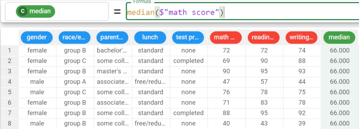
In the example here, we want to retrieve the median value of the math score attribute.
We type the following formula:
median($"math score").The median of the math score attribute is 66.
Example - median(column, group)
The following example uses the Students Performance dataset.
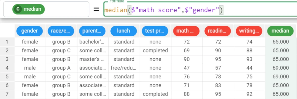
In this second example we want to group our results by the lunch attribute, so the formula will be:
median($"math score",$"gender").The results are as follows: * The median value of the math score for female students is 65. * The median value of the math score for male students is 69.
min
The min function is intended to retrieve the minimum value of an attribute.
The min function retrieves the minimum value of an attribute, eventually grouped, or if a list of attributes is provided in the column parameter it compares the various attributes retrieving the maximum value between them.
See also
The minimum (min) function only is available also by:
Selecting the column in the Data tab and finding the minimum in the Info row bar (for not nominal-like or date-like attributes only).
Dragging the attribute in the Apply‘s query panel.
Selecting the function in the Sheets.
Parameters
min(column, group)
Parameter |
Description |
column |
It identifies the column to which you want to apply the formula. The column parameter is mandatory. |
group |
It allows you to group the results by a certain column. |
Example - min(column)
The following example uses the Students Performance dataset.
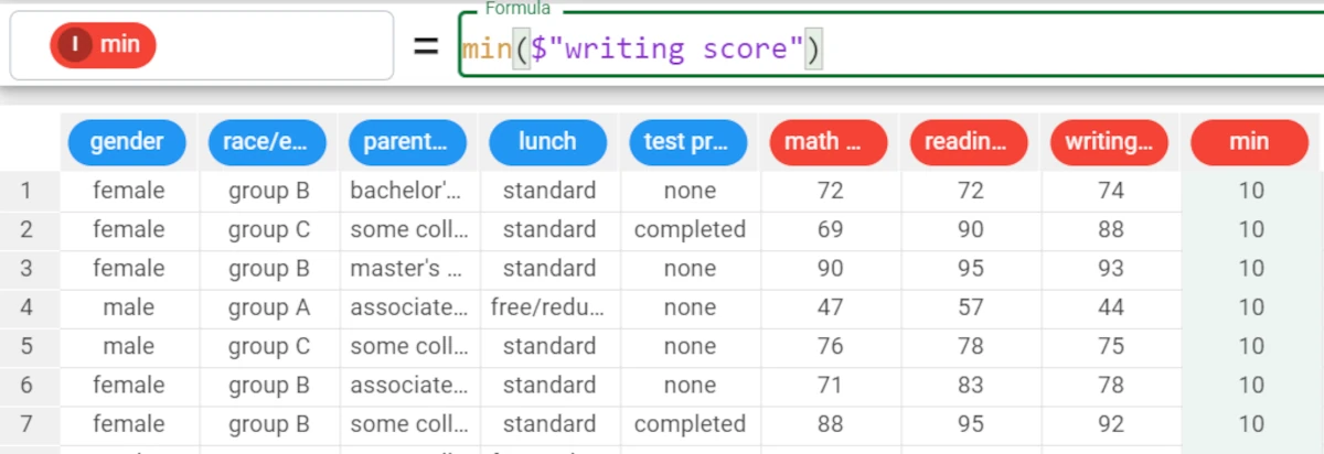
In the example here, we want to fill the min attribute with the minimum of the writing score attribute.
We type the following formula:
min($"writing score")and the function returns the lowest value for the writing score.
Example - min(column, group)
The following example uses the Students Performance dataset.
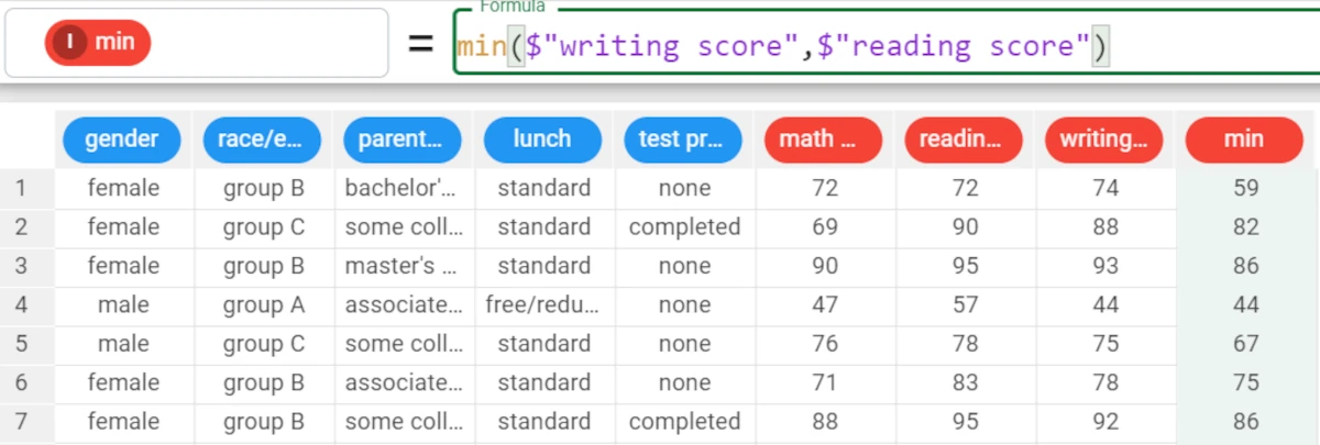
If we want to group our results by their reading score, the formula will be:
min($"writing score",$"reading score")and the function returns the lowest value for the writing score, grouped by the reading score.So the results will be: * The minimum writing score value associated with the 72 reading score is 59. * The minimum writing score value associated with the 90 reading score is 82.
Example - min((column1, column2))
The following example uses the Students Performance dataset.
In the example here, we want to compare the writing score and the reading score, and we want to retrieve the lowest value between them.
We write the following formula:
min(($"writing score",$"reading score")).The results are as follows: * In row 1, the minimum value between the writing score value (74) and the reading score value (72) is 72. * In row 2, the minimum value between the writing score value (88) and the reading score value (90) is 88 and so on.
min2
Danger
This function is deprecated for comparing attributes: use instead min((column1, column2)). This function is still useful to compare scalar values between them or scalar values with attributes.
The min2 function compares two elements and retrieves the minimum value between them.
Parameters
min2(elem1, elem2)
Parameter |
Description |
|---|---|
elem1 |
It identifies the element to which you want to apply the formula. The elem1 parameter is mandatory. |
elem2 |
It identifies the element to which you want to apply the formula. The elem2 parameter is mandatory. |
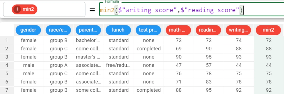
Example - min2(elem1, elem2)
In this example we want to compare the value
Truewith the value2We then write the formula
min2(True, 2)The result will be
1in all the rows sinceTrueis automatically converted in the number1which is lower than2.
mode
The mode is the most frequent value in an attribute.
For example, the mode in the list [23; 26; 26; 26; 4; 7; 7; 98] is 26.
See also
The mode function is available also by:
Selecting the column in the Data tab and finding the minimum in the Info row bar (for continuous values only).
Dragging the attribute in the Apply area of the Data Manager’s query panel.
Selecting the function in the Sheets tab of the Data Manager.
Parameters
mode(column, group, usemissing)
Parameter |
Description |
|---|---|
column |
It identifies the column to which you want to apply the formula. The column parameter is mandatory. |
group |
It allows you to group the results by a certain column. |
usemissing |
A Boolean which indicates whether missing values should be considered or not in the computation of the statistics. The default value, if not otherwise specified, is True. |
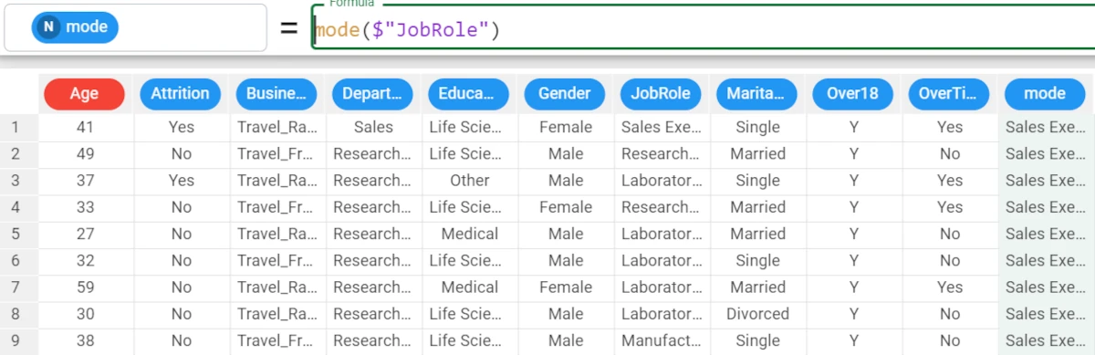
Example - mode(column)
The following example uses the HR employee attrition dataset.
In the example here, we want to retrieve the mode of the Job Role attribute.
We write the following formula:
mode($"JobRole").The mode of the Job Role attribute is Sales Executive.
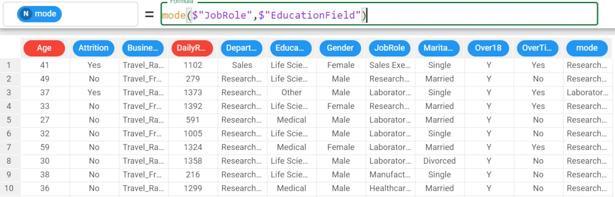
Example - mode(column, group)
Then, we want to group our results by the Education Field attribute, and to have a 0 when a value is missing.
So the formula is:
mode($"JobRole",$"EducationField").The results are as follows: * The mode of the Job Role for the Life Sciences education field is Research Scientist. * The mode of the Job Role for the Other education fields is Laboratory Technician.
movMean
The moving mean (also known as moving average) analyzes data points by creating a series of averages of different subsets of the chosen column.
Returns the moving average of the column, evaluated on the lag continuous rows, computed according to groups defined by the group parameter if required.
Each row represents the first value of the lags in which the column will be divided.
Similar operations are available also in the Moving Window task.
Parameters
movMean(column, lag, group, front)
Parameter |
Description |
|---|---|
column |
It identifies the column to which you want to apply the formula. The column parameter is mandatory. |
lag |
It is the number of continuous rows used to evaluate the moving average. The lag parameter is mandatory. |
group |
It allows you to group the results by a certain column. This is an optional parameter. |
front |
it is an optional parameter. If not specified, |
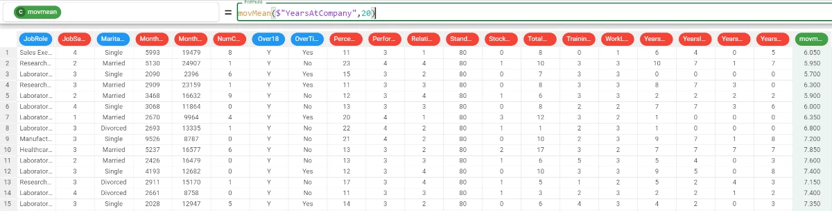
Example - movMean(column, lag)
The following example uses the HR employee attrition dataset.
In the example here, we decided to calculate the moving mean of the Years at Company attribute, with a lag of 20 rows.
We write the following formula:
movMean($"YearsAtCompany",20).
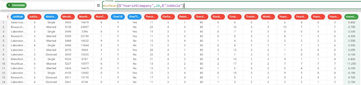
Example - movMean(column, lag, group)
If we want to go on with our analysis we can add a group parameter, by which our results will be grouped.
We decided to group the values by the Job Role attribute, so the formula becomes:
movMean($"YearsAtCompany",20,$"JobRole").The results are as follows: * For the Sales Executive job role, the moving mean of the Years at Company attribute is 9.450. * For the Research Scientist job role, the moving mean of the Years at Company attribute is 4.750.
pearson
The pearson function returns the Pearson coefficient between column1 and column2, evaluated within groups defined by the group parameter if required.
The pearson coefficient represents the relationship between two continuous variables.
Hint
The Pearson coefficient ranges from -1 to +1, where:
-1 represents a negative correlation
+1 represents a positive correlation
See also
The Pearson function is available also by selecting it in the Sheets tab of the Data Manager.
Parameters
pearson(column1, column2, group)
Parameter |
Description |
|---|---|
column1 |
It identifies the first column to which you want to apply the formula. The column1 parameter is mandatory. |
column2 |
It identifies the second column to which you want to apply the formula. The column2 parameter is mandatory. |
group |
It allows you to group the results by a certain column. |
Example - pearson(column1, column2)
The following example uses the Bike Sales dataset.
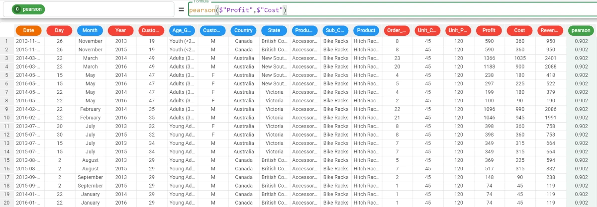
In the example here, we would like to retrieve the Pearson coefficient between the Profit and Cost attributes.
We write the following formula:
pearson($"Profit",$"Cost").The value of the Pearson coefficient is 0.902, so the result is considered positive.
Example - pearson(column1, column2, group)
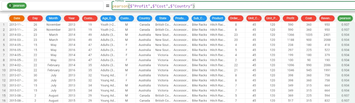
If we want to go further with our analysis, we can group our results by a specific attribute values.
In the example here, we decided to group out results by the Country attribute, so the formula becomes:
pearson($"Profit",$"Cost",$"Country").The results are as follows: * The Pearson coefficient between the Cost and Profit in Canada is 0.937; * The Pearson coefficient between the Cost and Profit in Australia is 0.934, and so on.
quantile
The quantile function returns the quantile of the column, evaluated within groups defined by the group parameter if required. A column of weights can also be defined.
Quantiles are cut points dividing a range of probability distribution into intervals with equal probabilities.
Parameters
quantile(column, quant, group, weights)
Parameter |
Description |
|---|---|
column |
It identifies the column to which you want to apply the formula. The column parameter is mandatory. |
quant |
It is the percentile. The quant parameter is mandatory. |
group |
It allows you to group the results by a certain column. |
weights |
It defines the importance of a certain attribute. |
Example - quantile(column, quant)
The following example uses the HR employee attrition dataset.
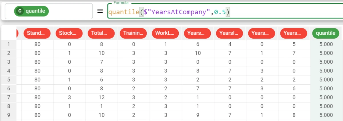
In the example here, we want to retrieve the quantile of the Years at Company attribute.
We write the following formula:
quantile($"YearsAtCompany",0.5). The 0.5 parameter indicates intervals from 0 to 5. The quantile for the Years At Company attribute with a 0.5 percentile is 5.
Example - quantile(column, quant, group=group, weight=weight)
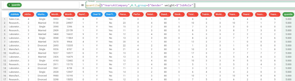
If we want to be more precise in our analysis, we can decide to group our results by a certain attribute’s values and to add more weight to another attribute.
For example, we want our values to be grouped by the Gender attribute, and that the Job Role attribute has more weight.
The formula becomes:
quantile($"YearsAtCompany",0.5,group=$"Gender",weight=$"JobRole"). In this case, the results don’t change.
roc
The roc function calculates a performance indicator, the AUC, that is the area under the curve defined by the column and the attclass.
The default value for the class attribute (if more than two values are present) can be specified as the optional parameter defclass. All computation can be performed according to the groups defined in the group parameter.
Hint
The AUC value ranges from 0 to +1, where: * 0 indicates the worst performance indicator * +1 indicates the best performance indicator.
The roc curve is also available in the Sheets tab of the Data Manager.
Parameters
roc(column, attclass, defclass, group)
Parameter |
Description |
|---|---|
column |
It identifies the column to which you want to apply the formula. The column parameter is mandatory. |
attclass |
It identifies the column to which you want to apply the formula. It is a nominal attribute. The attclass parameter is mandatory. |
defclass |
It is the default value for the class attribute. |
group |
It allows you to group the results by a certain column. |
weights |
It defines the importance of a certain attribute. |
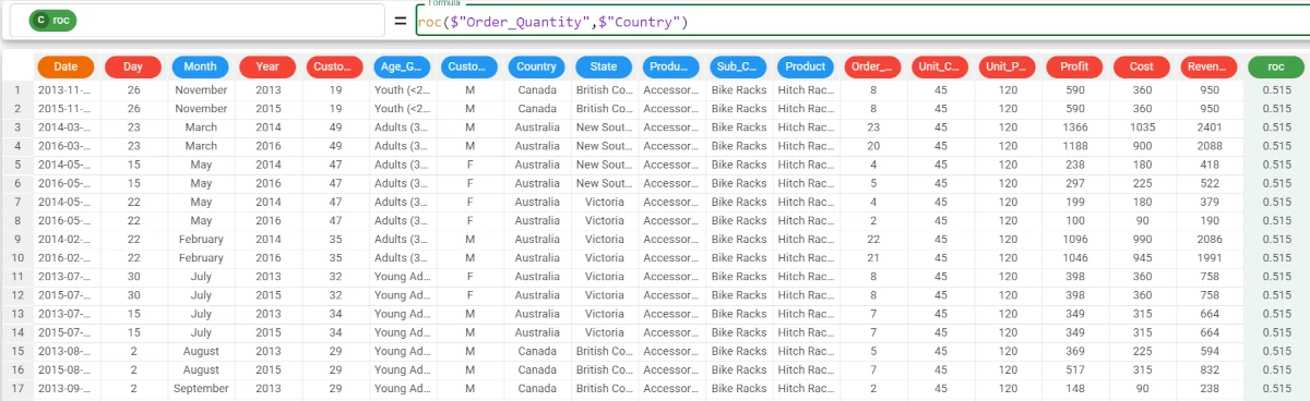
Example - roc(column, attclass)
The following example uses the Bike Sales dataset.
In the example here, we want to retrieve the AUC value for the Order_Quantity attribute with the Country target.
The formula to write is:
roc($"Order_Quantity",$"Country").We can double-check the result in the Statistics tab, by dragging the _Order_Quantity_ attribute onto the Var_1 area and the Country attribute onto the Y area.
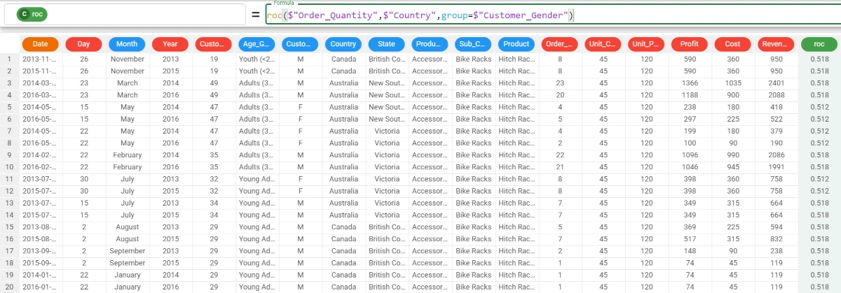
Example - roc(column, attclass, group=group)
If we want to group our results, we can add the group parameter, that, if the defclass is not defined, must be written as
group=$"att".We want to group our results by the Customer_Gender attribute, so the formula becomes:
roc($"Order_Quantity",$"Country",group=$"Customer_Gender").The results are as follows: * The AUC value for the Male customers is 0.518 * The AUC value for the Female customers is 0.512.
std
The standard deviation is a statistical function which measures the dispersion of a dataset relative to its mean, and it is the square root of the variance.
The higher the standard deviation, the furthest values are far from the expected standard value.
See also
The standard deviation is also available by:
Parameters
std(column, group)
Parameter |
Description |
|---|---|
column |
It identifies the column to which you want to apply the formula. The column parameter is mandatory. |
group |
It allows you to group the results by a certain column. |
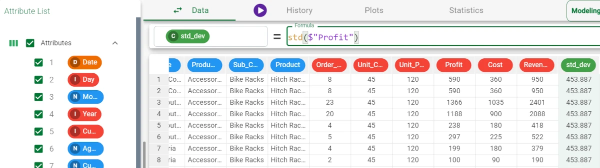
Example - std(column)
The following example uses the Bike Sales dataset.
In the example here, we want to retrieve the standard deviation of the Profit attribute.
We add a new attribute. We write the following formula:
std($"Profit")
Example - std(column, group)
If we want to be more precise with our analysis, we can add the group parameter.
Here we want to group the results by the Country values, so the formula will be:
std($"Profit",$"Country").The results are as follows: * The standard deviation for the Profit in Canada is 451.913. * The standard deviation for the Profit in Australia is 430.6.

variance
The variance function returns the variance of the column, evaluated within groups defined by the group parameter if required.
The variance is a measure of dispersion, which displays how a set of values is far from their average value.
See also
The variance function is also available by:
Parameters
variance(column, group)
Parameter |
Description |
|---|---|
column |
It identifies the column to which you want to apply the formula. The column parameter is mandatory. |
group |
It allows you to group the results by a certain column. |
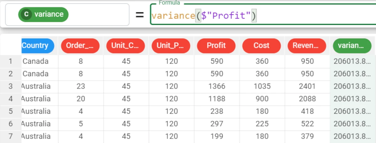
Example - variance(column)
The following example uses the Bike Sales dataset.
In the example here, we want to retrieve the variance of the Profit attribute.
We add a new attribute and write the following formula:
variance($"Profit").The variance for the Profit attribute is 206013.811
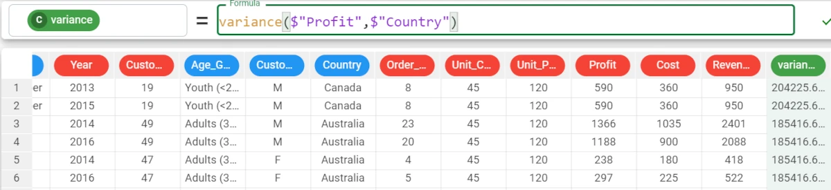
Example - variance(column, group)
If we want to have a more specific analysis, we can add the group parameter to the formula.
In the example, we want our results to be grouped by the Country attribute.
The formula becomes:
variance($"Profit",$"Country").The results are as follows: * The variance for Canada is 204225.686. * The variance for Australia is 185416.613.