Mixed Integer Linear Programming

Linear programming is used to obtain the optimal solution for a problem by representing a real life scenario as a mathematical model with defined constraints.

Typical linear problems consist in finding the optimal values for a set of attributes (inputs) in order to minimize costs or maximize performance levels.

Rulex provides the Mixed Integer Linear Programming task, which means that:

• the model and the constraints must be expressed as linear combinations of the inputs

• the optimal values for the inputs can either be expressed as a rounded-up integer or as a continuous value.

The Mixed Integer Linear Programming task is divided into three tabs:

• the Options tab

• the Solutions tab

• the Results tab

---

The Options tab

The Options tab is divided into four areas:

• the Available attributes, containing the dataset’s attributes.

• the Table mode area, specifying the format of the input table: once the input format is chosen, the Attribute area varies according to it.

  • Normal: each row of the input table is considered as a single constraint and a column for every variable used in the analysis.

  • Sparse: in the input table, there will be a row for each coefficient different from 0, and it will contain 3 columns (mandatory). This mode allows a smaller dataset as input, so it requires less memory to complete the computation.

• The Attribute area, which adapts according to the chosen table mode.

  • If the Normal Table mode has been chosen, the following options are available:

    • Coefficients for integer solutions (INTEGER/CONTINUOUS): drag the coefficient attributes that will be used in the calculation, if the results must be provided as an integer. Instead of manually dragging and dropping attributes, they can be defined via a filtered list.

    • Coefficients for continuous solutions (INTEGER/CONTINUOUS): drag the coefficient attributes that will be used in the calculation, if results can be provided as a continuous value. Instead of manually dragging and dropping attributes, they can be defined via a filtered list.

    • Attribute for constraint (and cost) types: select the attribute (column) which contains the row type, which can be:

      • cost, objective, c, o (for the row that contains the cost function coefficients)

      • == (for equalities, constraints)

      • >=, >, etc. (for comparative constraints, such as greater than, equal to etc.)

      • min, max (for minimum and maximum values respectively)

    • Attribute for right hand side values: select the attribute (column) that contains the constants for the constraint rows.

  • If the Sparse Table mode has been chosen, the following options are available:

    • Attribute for row value: select the attribute containing a label to identify which constraint you are referring to. Its type can be both ordinal or nominal.
      If the attribute type is Nominal, the values can be:

      • min, minimum (for the row containing the minimum value)

      • max, maximum (for the row containing the maximum value)

      • type (for the row containing the variable type)

      • cost, obj, objective (for the row containing the cost function coefficients)

      • sol, solution (for the row containing the solution value)

      • the constraint name

      If the attribute type is Integer, the values can be:

      • -2 (for the row containing the minimum value)

      • -1 (for the row containing the maximum value)

      • 0 (for the row containing the variable type)

      • -3 (for the row containing the solution value)

      • the constraint_ind, which is an integer number greater than 0.

    • Attribute for col value: select the attribute containing the output attribute’s name. Its type can be both ordinal or nominal.
      If the attribute type is Nominal, the values can be:

      • >=, >, <=, <, ==, = (for the constraint type)

      • the var_label, which identifies the variable

      If the attribute type is Integer, the values can be:

      • the var_ind, which is an integer number greater than 0

      • -2, -1, 0 (indicating respectively >=, >=, ==)

    • Attribute for coefficient value: select the attribute containing the coefficient used to make the analysis. Its values can be:

      • the minimum, maximum, cost, solution, rhs values

      • 0, 1, 2 for the variable type (indicating respectively a continuous, integer or binary variable)

• The configuration options area, which contains the following choices:

  • Optimization mode: select whether you want your solution to Maximize or Minimize the outcome.

  • Maximum execution time (seconds): specify for how many seconds the task can run. If not specified, no time limits are set.

  • Overwrite data with solution coefficients: if selected, the outcoming data will be transmitted to the consecutive tasks. If not selected, the results will be saved within the Mixed Integer Linear Programming task only, and the input dataset will be transmitted as output.

  • Maximum number of iterations: specify how many times the task can be run. If not specified, no limits on the number of iterations are set.

  • Solver used for optimization: select the solver which will be used for the optimization operation. Possible solvers are:

    • Coin-Or

    • Symphony

    • Naive (Rulex proprietary solver, it is faster than the others, but it provides a less accurate result)

  • Stop at first feasible solution: if selected, the optimization operation stops when a solution satisfying all the constraints is found. It might be possible that the solution found is not the best one.

  • Add feasible column in dataset: if selected, a binary column, called ‘Feasible’ is added to the dataset. The value ‘True’ indicates that the solution is feasible, while the value ‘False’ indicates that the solution is unfeasible.

---

The Solutions tab

The Solutions tab displays the generated solutions in a spreadsheet format.

---

The Results tab

The results tab provides information on the computation. It is divided into two sections:

• In the General Info section, you will find:

  • The Task Label, which is the task’s name on the interface.

  • The Elapsed time, which indicates how long it took to complete the computation.

  • The Optimum value of the cost function,

---

Example - Normal table mode

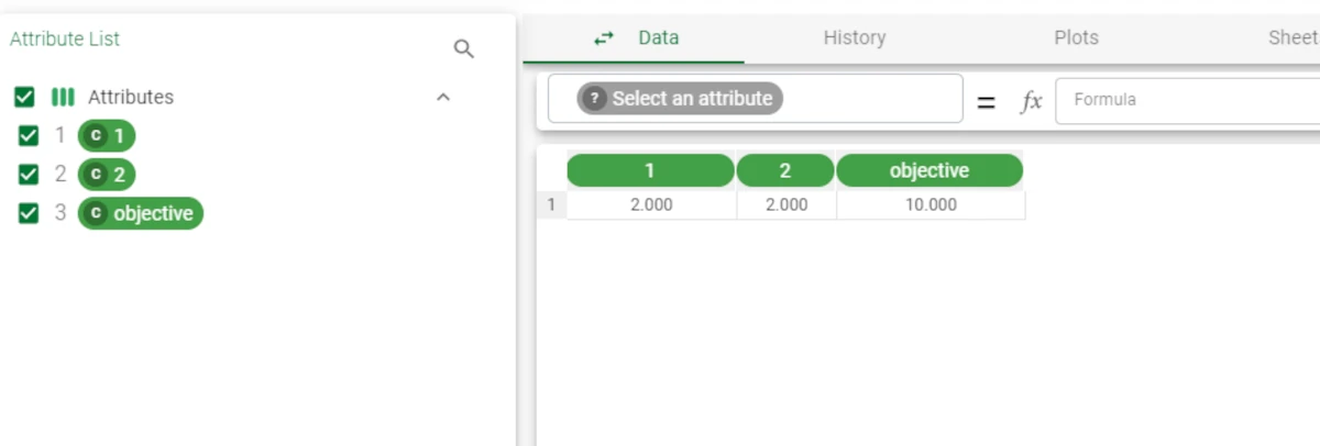
The following example uses the yogurt dataset.

The basic scenario used in this example involves a small family-run farm factory where two types of yogurt are produced:

• deluxe strawberry yogurt, which contains two units of yogurt and two units of strawberries, and produces a profit of 3 euros per unit of finished yogurt.

• super saver yogurt, which contains three units of yogurt and one unit of strawberries, and produces a profit of 2 euros per unit of finished yogurt.

There are currently 15 units of yogurt and 10 units of strawberries in stock, and at least two units of each type of yogurt must be produced to meet current orders.

Objective: The factory wants to maximize its profits by finding out the optimal amount of deluxe and super saver yogurt to make with its currently available stock.

The information in the scenario can be mathematically expressed as follows:

• The amount of deluxe yogurt to produce = x

• The amount of saver yogurt to produce = y

• The maximum profit = z

• Consequently z = 3x (profit multiplied by the amount produced) + 2y

Our constraints are as follows:

• Strawberry stock constraint: 2x + y <= 10

• Yogurt stock constraint: 2x + 3y <= 15

• Minimum values:

  • x >=2

  • y >=2

• After having imported the dataset, add a Mixed Integer Linear Programming task to the flow and link it to the import task.

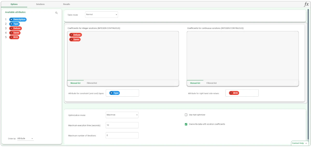
• Double-click the task and set the following parameters:

  • Table mode: Normal

  • Coefficients for integer solutions: drag the Deluxe and Saver attributes.

  • Optimization mode > Maximize, as we want to maximize our profits.

  • Attribute for constraint (and cost) types > specify the Type column, which contains the functions.

• Attribute for right-hand side values > specify the RHS column, which contains the constants.

• Maximum execution time > specify a maximum of 10 seconds.

• Maximum number of iterations > do not provide a maximum number of iterations.

• Select Overwrite data with solution coefficients to view the solution results in the successive Data Manager task.

• Drag the attributes for the two types of yogurt onto the Coefficients for integer solutions target list, as we want the solution to be expressed as whole units, and not continuous values.

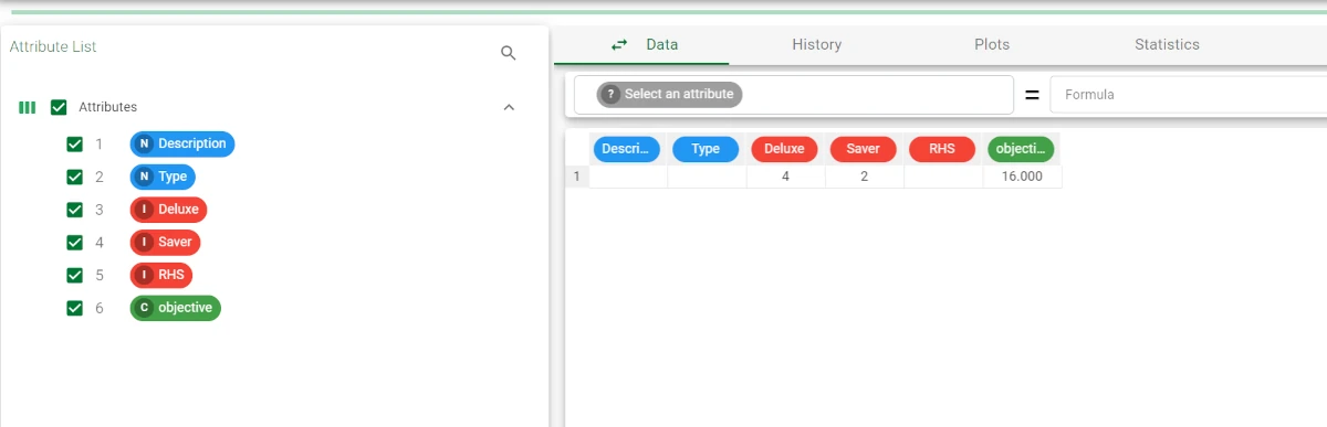
• After saving and clicking Compute to start the analysis, the solution to our problem can be viewed in the Data Manager task.

• The maximum profit is 16 euros (objective), if we produce (and obviously manage to sell):

  • 4 units of deluxe strawberry yogurt

  • 2 units of super saver strawberry yogurt.

The same information can be viewed directly in the Solutions tab of the Mixed Integer Linear Programming task if we select Overwrite data with solution coefficients.

---

Example - Sparse table mode

The following example uses the Sparse dataset.

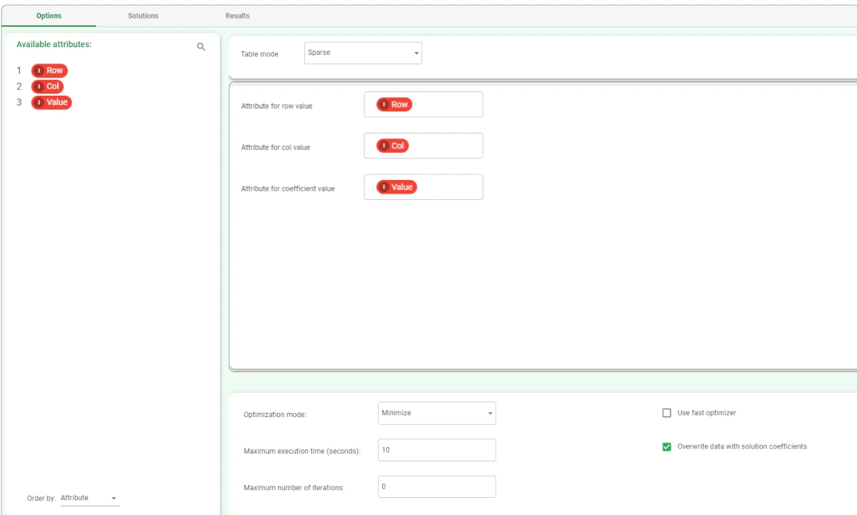
• After having imported the dataset, drag a Mixed Integer Linear Programming task onto the stage and configure it as follows:

  • Table mode: Sparse

  • Attribute for row value: Row

  • Attribute for col value: Col

  • Attribute for coefficient value: Value

  • Optimization mode: Minimize

  • Maximum execution time (seconds): 10

  • Maximum number of iterations: 0

  • check the Overwrite data with solution coefficients checkbox

• Save and compute the task.

• The solution to the problem can be visualized in the Data Manager task: add a Data Manager task to the flow and link it to the Mixed Integer Linear Programming task.

• The solution headers are the var_ind which have been specified in the original dataset.